
Noether’s First Theorem
Published:
Let’s begin with an example from electromagnetism; actually, it’s really just a kinematic observation. Say we have a solid region $W \subset \mathbb{R}^3$ with a closed, piecewise smooth boundary $S$. There may be charged particles in $W$ and we note that if $\rho$ is the time-dependent charge density (which has units charge/volume), then the total charge is $Q(t) = \iiint_W \rho \, dV$. If we take a time derivative, we’d have $\frac{dQ}{dt} = \iiint_W \partial_t \rho\, dV$. Now, if the charges inside $W$ were to teleport around, the total charge would be unaffected but it’s unclassical for particles to teleport around instantly; i.e. we assume locality. So we’d like to stipulate that the only way for the total charge to change is if charged particles enter/leave through $S$ in a continuous way. So we’d have moving charges which create current $I$. Set $\frac{dQ}{dt} = -I$; the minus sign is just to align with the outward pointing orientation $\hat{n}$ of $S$; so if charges leave, then the total charge is decreasing and we’ll say the current is positive in the $\hat{n}$ direction.
Anyways, let $J = \langle J_1,J_2,J_3 \rangle$ be a time-dependent vector field representing the current density (so the units are charge/(area x time)). It’s a vector field as opposed to a scalar function like $\rho$ since current can point in any direction. Then $I = \iint_S (J \cdot \hat{n})\, dA$ because this integral measures how much current is passing through $S$. The divergence $\nabla \cdot J = \partial_x J_1 + \partial_y J_2 +\partial_z J_3$; if we integrate it over the volume $W$, we’d have $\iiint_W \nabla \cdot J\, dV = \iint_S (J \cdot \hat{n})\, dA$. This works for any $W$, even very small volumes and we’re using a case of the (generalized) Stokes Theorem known as the Divergence Theorem.
Since what we said above works for tiny volumes $W$, we can basically say it happens at every point! So we obtain a continuity equation $\partial_t \rho + \nabla \cdot J = 0$. This equation represents conservation of charge since if we integrate over any volume, we’d get that the change in total charge can only occur continuously via charged particles moving past the boundary.
For magnetic fields $B$, we have a similar equation but it is $\nabla \cdot B =0$ because there is no net gain or loss; classical magnets always have a north and south pole and the field lines leaving it are balanced by the field lines coming in.
More generally, a conserved current $j^\mu = (j^0,j^1,j^2,j^3)$ is a vector field in Minkowski $\mathbb{R}^{1,3}$ that satisfies a kind of continuity equation: $\partial_\mu j^\mu := \partial_0 j^0 -\sum_{i=1}^3 \partial_i j^i =0$. Here, the index 0 is the time component and the others are spatial.
If we have a volume $W \subset \mathbb{R}^3$ such that there is no net current through the boundary surface, then we’d get a conservation law similar to before. We’d have $\partial_0 Q = \iiint_W (\sum^3_{i=1} \partial_i j^i) \,dV = \iiint_W \partial_0 j^0$; the first equality is like above and the second is by using this new version of the continuity equation. The triple integral, by the Divergence Theorem, is $\iint_{\partial W} (j \cdot \hat{n})\, dA$. If there is no net current at the boundary as we assumed, then the integral is 0 and so again, we’ll have that $\partial_0 Q = 0$; i.e. the charge is conserved so we have a conservation law.
Stating Noether’s First Theorem
We’ll now given an informal statement of Emmy Noether’s theorem: every differentiable symmetry of the action of a classical physical system with conservative forces has a corresponding conservation law.
In the context of what we were saying above, another statement is: To every differentiable symmetry of the action functional, there exists a locally conserved current. From the conserved current, one can then get the conserved quantity. Note that above, we were not discussing any symmetries. So what do we require of the action functional? It’s usually written like
\[S[\gamma] = \int L(\gamma(x),\partial \gamma(x),x)\, dx\]where $\gamma$ is a path and $L$ is a Lagrangian density depending on a the path, finitely many derivatives of the path, and the parameter of the path. A symmetry of this action is simply some kind of transformation we can apply to the path $\gamma$ where action on the newly transformed path is the same as the original plus a boundary term. For example if $T$ is the transformation, then $S[T(\gamma)] = S[\gamma] + B$ where $B$ is the boundary term; it only depends on the behavior of the fields on the boundary. Like above, where the triple integral on the bulk $W$ is equal to a surface integral on the boundary $\partial W$. The symmetries map critical points to critical points, hence solutions of the equations of motion to solutions.
Also, the current is locally conserved meaning we have a local continuity equation like the one above. Something like $\partial_\mu j^\mu(x) = 0$. Such a current $j$ exists point wise but not necessarily globally.
Remark: It’s important to note that these are classical, not quantum systems.
Revisiting the Example
So above, we had the continuity equation (slightly rewritten) $\partial_t \rho =- \nabla \cdot J$ which tells us that the way the charge density changes is equal to minus the divergence of the current density.
An alternative way to obtain this is to introduce two of Maxwell’s Equations (all the terms have been introduced above):
\[\nabla \cdot E=\rho, \hspace{15mm} \nabla \times B - \partial_t E=J.\]Take the divergence of the second equation: $\nabla \cdot (\nabla \times B) - \partial_t(\nabla \cdot E)=\nabla \cdot J$.
The first term vanishes (it’s essentially $d^2 = 0$) and we substitute $\rho = \nabla \cdot E$ to get $\partial_t \rho + \nabla \cdot J=0$.
We could instead write down a Lagrangian density for electromagnetism. If we have a scalar field $\phi:\mathbb{R}^{1,3} \to \mathbb{C}$, the density is $L = \partial_\mu \phi^* \partial_\mu \phi - m^2 |\phi|^2$; here $\phi^*$ is the complex conjugate. Multiplying by $e^{i\theta} \in U(1)$ doesn’t do anything to $L$ so then integrating $L$ will also not be impacted by this transformation of $U(1)$. The derivation of the conserved current is a bit more involved but we get the Noether current $j^\mu = i(\phi \partial^\mu \phi^* - \phi^* \partial^\mu \phi)$. Applying $\partial_\mu$, we get some cancellation of terms and arrive at
$\partial_\mu j^\mu=i(\phi \square\phi^*-\phi^* \square \phi)$ where $\square$ is the wave or d’Alembert operator. Using the equations of motion $(\square + m^2)\phi = 0,(\square + m^2)\phi^*=0$, we get total cancellation and end up with just the continuity equation $\partial_\mu j^\mu=0$. On the other hand, if we unpack $j = (\rho,J)$, then the continuity equation is once again $\partial_t \rho + \nabla \cdot J=0$.
The symmetries here from $U(1)$ are a global symmetry; it doesn’t matter where $x \in \mathbb{R}^{1,3}$ is, the action of the scalar field $\phi(x)$ is the same. It’s important to distinguish this kind of global symmetry from internal symmetries even if sometimes, the same Lie group appears. Noether’s 2nd Theorem deals with these internal symmetries.
Examples of Symmetries and Conserved Quantities
Here is a table with some symmetries and conserved quantities in the context of Noether’s 1st Theorem.
| Symmetry | Conserved Law |
|---|---|
| Spatial Translation | Total Momentum |
| Spatial Rotation | Total Angular Momentum |
| Phase Rotation | Total Probability (mass) |
| Gauge Transformation | Total Charge |
| Time Translation | Total Energy |
| Diffeomorphisms in General Relativity | Stress-Energy |
One of the things to note here is that these are still about local conservation. In order for energy conservation to occur globally, we need a global time translation symmetry. But in general relativity, there simply is no such global time translation; time isn’t even globally defined in a distinct way from space. So in fact, energy doesn’t need to be conserved within the entire universe! See this video on the topic.
Sketch of a Proof
The Lagrangian viewpoint is very powerful so that’s the approach we’ll take. With many physical systems, we can write down a Lagrangian action $S(u)$ which tells us the action for a trajectory $u$. This trajectory represents a particular evolution of the system over time, say, on $[0,T]$. The way this can go, for example is to take a Lagrangian density $L(t,u,\dot{u})$ which depends on time, $u$, and the time derivative of $u$ (in other settings, there may be further dependence on higher derivatives of $u$ or other factors). Then, the action is $S(u)=\int^T_0 L(t,u,\dot{u})\, dt$.
A critical point of $S$ should be viewed similarly to finite dimensions; the “instantaneous rate of change of $S$ at a critical point $u$ is 0.” It turns out that $u$ is a critical point if and only if it is a solution to the Euler-Lagrange equations. These solutions, classically speaking, represent actual physical trajectories. So we’re able to understand how the system evolves (once we have initial and final conditions); it evolves via such $u$.
So now, we outline Feynman’s argument (I learned this from Terrence Tao). If $\tilde{u}$ is a small perturbation of $u$ and they both have the same initial and final states, then $S(\tilde{u}) \approx S(u)$. If the initial and final states of $\tilde{u}$ are also slightly perturbed, then we’d have $\tilde{u}(0)=u(0)+ \delta u(0)$ and $\tilde{u}(T)=u(T) + \delta u(T)$. Using chain rule and integration by parts, we’d find that $S(\tilde{u}) \approx S(u) + D(\delta u(T))-D(\delta u(0))$. The picture here shows three situations; the first two are what we just described.
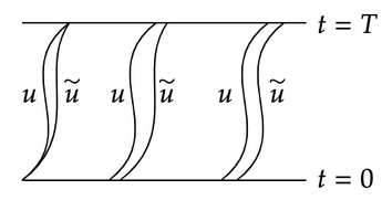
Next, suppose that $\tilde{u}$ is a perturbation of $u$ by a symmetry (so this is a local action by a differentiable symmetry because it’s small); that’s the third situation in the picture. Since it’s a symmetry of the action, $S(\tilde{u}) = S(u)$. But also, $S(\tilde{u}) \approx S(u)+D(\delta u(T))-D(\delta u(0))$. So we’re forced to conclude that $D(\delta u(T))=D(\delta u(0))$; i.e. something is conserved between time 0 and time $T$. $\square$
Relation between Noether’s First Theorem and Heisenberg Uncertainty
One of the things we note about Noether’s 1st theorem is that the conserved quantity for spacial translations (change in position) is momentum and the conserved quantity for temporal translations is energy. Both of these pairs have some kind of Heisenberg Uncertainty relationship though time is also tricky to understand in quantum theory. But anyways, this is not an accident. I drew the following from this physics.stackexchange post.
Noether’s 1st Theorem and the Heisenberg Uncertainty Principle (HUP) are related by the following notions.
- From Hamiltonian mechanics, every dynamical variable can be interpreted as an infinitesimal generator of some canonical transformation (a symmetry). That is, one of the equations of motion is $\frac{df}{dt} = \{H,f\}$ where $H$ is the Hamiltonian and we have an (antisymmetric) Poisson bracket. But we can also use $\{-,f\}$ to define a vector field $X_f$ which is the infinitesimal generator of a “canonical transformation” mentioned. Moreover, if $j$ Poisson commutes with $H$, then the equation of motion is saying that $\frac{dj}{dt}=0$; i.e. it is unchanged over time by the dynamics and hence, conserved. We could call this the Noether charge.
- In quantum mechnics, every skew-Hermitian operator generates a unitary transformation. That’s because $\text{Lie}(U(n))=\mathfrak{u}(n)$ are skew-Hermitian and the exponential map generates unitary matrices. If we do canonical quantization, then the Noether charge which Poisson commuted with the Hamiltonian will be sent to something that Lie commutes with the quantum Hamiltonian.
The Heisenberg principle is true of any variable/observable (an operator) with a continuous spectrum and the infinitesimal generator of translations in that variable. This is just because these variables always have a dual with which it does not commute. Position and momentum, angle and angular momentum, charge and phase, these are all conjugates in classical mechanics.
Example: The position operator $\hat{q}(f) = xf$ (multiply by $x$) and the momentum operator is $\hat{p}(f)=i\hbar\frac{d}{dx}(f)$ which is an infinitesimal generator if we think of $\frac{d}{dx}=\partial_x$ as a vector field (which are equivalently viewed as derivations). Then $[\hat{p},\hat{q}] (f)=-i\hbar f$ which is nonzero. Above, we said we need a skew-Hermitian operator to generate a unitary transformation. Indeed, the $i$ on $i\hbar\frac{d}{dx}$ ensures skew-Hermitianess. If we apply an exponential to generate a unitary transformation, we get $\hat{D}_a = \exp(-\frac{i}{\hbar}a\hat{p})$. This is the operator that spatially displaces a wavefunction in the $x$ direction by an amount $a$.
Noether’s 1st theorem states that when we have a symmetry of a certain variable (say the symmetries are a Lie group $G$), the infinitesimal generators of those symmetries (which live in the Lie algebra $\mathfrak{g}$) is conserved. So translations in $x$, translations in angle, and translations in phase give conservation of momentum, angular momentum, and charge. But these generators obey the HUP with their conjugate variables.
Example: The Lie group $\mathbb{R}^n$ acts by spatial translations (position) and the infinitesimal generators are the left-invariant vector fields living in $\text{Lie}(\mathbb{R}^n)$; these are derivations which act on functions $f:\mathbb{R}^n \to \mathbb{R}$.
Noether’s Theorem in Quantum Systems
This section is built off this post. Noether’s theorem doesn’t always hold for quantum systems. In QFT, for example, we’ll integrate over all paths, not just those that solve the equations of motion: $\int_\mathcal{P} \exp(-\frac{i}{\hbar}S)\, \mathcal{D}x$.
Of course, the intuition is that the classical paths contribute the most but that can be enough to make it so that having symmetries does not guarantee conserved quantitites. Also, symmetries of the Lagrangian action do not necessarily give symmetries for the quantum action.
Above, I mentioned that the Noether charge Poisson commutes with the Hamiltonian and thus, is sent to something that commutes with the quantum Hamiltonian after canonical quantization. But canonical quantization is kind of a mathematical heuristic; very powerful but not completely correct and also not completely well-defined between classical and quantum theories. This leads to some interesting phenomena.
For instance, we have quantum anomalies. A standard example is from electroweak theory. There is a chiral anomaly where the classically conserved Noether current is not conserved in the quantum theory. The answer in the post contains the quote: “Anomalies of global symmetries are interesting but non-threatening phenomena, anomalies of gauge symmetries (local symmetries) are an obstruction to having a well-defined quantum theory, and the requirement that the total anomaly of a gauge symmetry must vanish is a powerful constraint in model building.” What this is saying is that if we have anomalous gauge (local) symmetries, it prevents us from consistently quantizing the theory in the first place so they “break” the entire theory. Dan Freed has a concrete way to frame anomalies in the language of obstruction theory; see here.
Remark: The definition for anomaly given by Green, Schwarz, Witten is pretty much framed in terms of Noether’s theorem. It is the breakdown of classical conservation law due to quantum-mechanical loop corrections. The quote above makes certain types of anomalies seem like disasters and anomalies of global symmetries as merely interesting. But for instance, the Higgs mechanism is from a global symmetry break which allows for hadrons to have nonzero mass.
Also, though Noether’s theorem doesn’t apply to quantum theories, you might wonder if the expectation value of the Noether current could be conserved. There is such a result, called the Ward-Takahashi identity. It says there is a relation between the symmetries and correlation functions.