Anomalies in Physics

This is a note based on a talk by Dan Freed entitled, “What is an Anomaly?” and the notes he posted for it. There are also slides from the talk. This is not my area of expertise and so any mistakes in here are due to me, not Dan Freed. The main slogan of the talk is the following: quantum theory takes place in projective geometry and an anomaly, mathematically speaking, can be viewed as an expression of this projectivity.

Anomalies might be seen as a problem to overcome but in fact, can be a feature. For example, the anomalies associated with certain symmetry breaking gives rise to the Higgs mechanism. Anomalies can become a problem if one wants to quantize since quantization is “linearization” and it’s possible to have something projective that doesn’t arise from vector spaces. For example, it’s possible to have a bundle with $\mathbb{CP}^n$ as fiber yet, it’s not a projectivization of a complex vector bundle of rank $n+1$.

Freed also listed two myths and “mythbusters” for why the myths are not true:

• Myth 1: Anomalies are only caused by fermionic fields
• Mythbuster 1: The flavor symmetry of QCD is anomalous—indeed, that anomaly involves fermions—but the anomaly persists in the effective theory of pions, which is a bosonic theory
• Myth 2: Anomalies are only associated to symmetries
• Mythbuster 2: The theory of a free spinor field has an anomaly

We’ll now turn our attention to some mathematics; much of this note will be focused on math but with motivation from physics.

Projective Geometry

Let $W$ be a $\mathbb{C}$-vector space and $K$ be any 1-dim $\mathbb{C}$-vector space. Then we have canonical isomorphisms of projective spaces $\mathbb{P}(W)\to \mathbb{P}(W \otimes K)$. Since a point of the projectivization is a line in $W$, the map sends a line $L\mapsto L \otimes K$. We also have the canonical isomorphism $\text{End}(W) \to \text{End}(W \otimes K)$ sending $T \mapsto T \otimes \text{id}_K$.

Remark: Over any field, a linear transformation $A:W \to W$ induces a map $\mathbb{P}(A): \mathbb{P}(W)\to\mathbb{P}(W)$ since linear maps send lines to lines. For example, let $R_\theta:\mathbb{R}^2 \to \mathbb{R}^2$ rotate the plane by an angle $\theta$. Then the induced map is on $\mathbb{RP}^1$. When we identify $\mathbb{RP}^1$ with $S^1$, the map is $e^{2 i \theta}$. For example, if the linear map rotates by $\pi$, then the map on $\mathbb{RP}^1$ is the identity. The converse is not true. For example, consider a map on $\mathbb{FP}^n$ which has $n+1$ fixed points where the fixed points come from linearly independent vectors $v_1,…,v_{n+1}$ on $\mathbb{F}^{n+1}$. If this map came from a linear map, then the linear map must be a diagonal map, scaling each vector $v_i$ by some $\lambda_i$. If there is another fixed point (so $n+2$ fixed points), the last fixed point represents a line spanned by, say, $w = \sum a_i v_i$ (let’s assume all the $a_i \neq 0$). Since it’s a fixed point, the linear map scales $w \mapsto \lambda w = \lambda \sum a_i v_i$. But also, this should be sent to $\sum a_i \lambda_i v_i$ since it’s a linear map. So then $\sum a_i(\lambda-\lambda_i)v_i = 0$; because the $v_i$ form a basis, we conclude that all the coefficients are 0 and hence $\lambda_i = \lambda$. That is, the linear map would have to just be a scalar multiple of the identity and hence, induce the identity map on projective space. But of course, one can cook up maps on projective space with $n+2$ fixed points but are not the identity map. For example, on $\mathbb{CP}^1$, complex conjugation fixes $\mathbb{RP}^1$ which is infinitely many points but is not the identity map.

Projective Representations and Classifying Principal $\mathbb{C}^*$-Bundles

Back to the talk. A projective symmetry/map of $\mathbb{P}(W)$ is a map that does come from a linear map on $W$ and hence, it has a $\mathbb{C}^*$-torsor of lifts to linear maps of $W$. This fact is captured by the short exact sequence: $0 \to \mathbb{C}^* \to GL(W) \to_\pi PGL(W) \to 0$.

Now, if $G \to PGL(W)$ is an injective Lie group morphism, then $G$ has a faithful projective representation. Shortening notation a bit, we can use $\pi$ to pullback $G$ to $GL$ to get a faithful linear representation of a Lie group $\widetilde{G}$. Also, we shorten notation without worry because everything works in the $\infty$-dim case where $GL=\lim_{n\to \infty} GL(n)$; same for $PGL$. We get the following diagram:

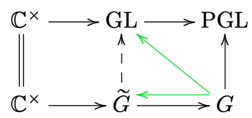
Now, we may ask whether the map $\psi:G \to PGL$ lifts to a map $G \to GL$ (the diagonal green arrow). Note that if we had a splitting $G \to \widetilde{G}$ (the left green arrow), we would get a lift. Conversely, say we had a lift $\tilde{\psi}:G \to GL$ so that $\pi \circ \tilde{\psi} = \psi$. Now, we always have a set-theoretic right inverse of surjective maps so there is such a right inverse $s$. Let’s give some names: we have $f:\widetilde{G} \to G$ and $\phi:\widetilde{G} \to GL$. So $\tilde{\psi}\circ f = \phi$. It’s a bunch of notation so let’s make a diagram.

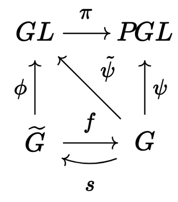
Then since $s$ is a splitting, $f\circ s = \text{id}_G$ and hence $\tilde{\psi} \circ f \circ s = \tilde{\psi} = \phi \circ s$. Then $\tilde{\psi}(gh) = \phi(s(gh))$; since we have some morphisms, the LHS is $\tilde{\psi}(g)\tilde{\psi}(h) = \phi(s(g))\phi(s(h)) = \phi(s(g)s(h))$. Because $\phi$ is injective, then $s(gh)=s(g)s(h)$ so the right-inverse $s$ is actually a group morphism.

Conclusion: We have a lift $G \to GL$ of an injective morphism $G \to PGL$ if and only there exists a splitting $s:G \to \widetilde{G}$.

Now, if we’re just speaking topologically, both horizontal sequences can be viewed as principal $\mathbb{C}^*$ bundles and hence, there are classifying maps $\Pi:PGL \to B\mathbb{C}^*$ and $\alpha:G \to B\mathbb{C}^*$. We could have had this whole discussion about $\mathbb{C}^* \to \widetilde{G} \to G$ as a principal bundle without referencing projective representations. But if we have the faithful Lie group morphism $G \to PGL$, then $\alpha$ factors through $PGL$ as $\alpha = \Pi \circ \psi$. When $\alpha$ factors in this way, it makes sense to speak of the “projectivity” of $\alpha$ and of course, the projectivity of $\alpha$ is equivalent to having the map $\psi:G \to PGL$ which is equivalent to $\widetilde{G}$ admitting an injective morphism to $GL$ with scalars $\mathbb{C}^*$ acting by multiplication.

So let’s return to the idea of having a lift $G \to GL$ which is equivalent to the existence of a splitting $s:G \to \widetilde{G}$. The splitting trivializes the principal bundle, giving us an isomorphism $\widetilde{G} \cong G \times \mathbb{C}^*$. This means the classifying map $\alpha$ is homotopically trivial.

Let’s study this $\alpha$ a bit more because it is this map which Freed calls an anomaly. From an obstruction theory standpoint, the obstructions to having a lift $G \to GL$ are cohomology classes in $H^k(G,\pi_{k-1}(\text{Fiber})) = H^k(G,\pi_{k-1}(\mathbb{C}^*))$. The only nontrivial homotopy group is when $k=2$ so the obstruction to the lift is a cocycle that in $H^2(G,\mathbb{Z}) = [G, B\mathbb{C}^*]$. Since we can interpret the cohomology classes in this way, we see that $\alpha$ is exactly the obstruction cocycle to lifting. I’m not sure why but Freed considers $H^2(G,\mathbb{C}^*)$ instead. Also, he says that if $G$ is not finite (or maybe not discrete), we need to use some other cohomology, not singular cohomology.

Anyways, if we have two splittings $s,t:G \to \widetilde{G}$, then we can take their ratios $s/t:G \to \mathbb{C}^*$; this is a character in representation theory. Hence, we can modify splittings by characters; i.e. the set of splittings is a torsor over characters. Now, Freed says that characters have cohomological interpretation as well; they are elements of $H^1(G,\mathbb{C}^*)$ (with the appropriate cohomology). One can think of characters as invertible linear representations. That is, a map $G \to \mathbb{C}^*$ acts on a 1-dim vector space to give a representation $L$ there is another character that gives a representation $K$ so that $L\otimes K$ is the trivial rep.

A slogan is that in QFT, projectivity is related to $H^2(G,\mathbb{C}^*)$ which is a shift of $H^1(G,\mathbb{C}^*)$, the invertible linear representations.

Question: How might we define a projective space without resorting to a linear space? Answer: Klein-Cartan say we can specify a geometry by its symmetries. Say we have a Lie group $H$ acting on $X$. We could, for example, take a right $H$-torsor $T$ and form $T \times_H X$. For example, with $\mathbb{CP}^n$, we can act on it by $PGL(n+1,\mathbb{C})$ to get complex geometry. Or enlarge it to a group that includes anti-holomorphic symmetries. Another option is to use $PU(n+1)$ to get Kähler structure or $PQ(n+1)$ which are isometries of the Fubini-Study metric.

Anyways, when we have a model geometry, we can work in families of them as well. Let $P \to S$ be a principal $H$-bundle where we allow $S$ to be a groupoid or a stack. For example, $S = */!/G$ would be just a single model geometry of $H$ acting on some space $X$ that is equipped with $G$-action.

Quantum Mechanics

Let $\mathcal{H}$ be a separable Hilbert space and $\mathbb{P}\mathcal{H}$ a space of pure states. We have a Hamiltonian $H \in \text{End}(\mathcal{H})$ and a probability function $p:\mathbb{P}\mathcal{H} \times \mathbb{P}\mathcal{H} \to [0,1]$ which sends a pair of lines $(L_0,L_1) \mapsto |\langle \psi_0,\psi_1 \rangle |^2$ where $\psi_i \in L_i$ has unit norm. We can also compute the amplitude and in fact, that’s preferable since the norm square of the amplitude is the probability.

For example, let $L_0$ be the initial state and $L_f$ the final. Let $t_0<t_1<…<t_n<t_f$ be real numbers and $A_1,…,A_n$ be endomorphisms of $\mathcal{H}$. Then the amplitude is: $\langle \psi_f, e^{i(t_f-t_n)H/\hbar}A_n…e^{i(t_2-t_1)H/\hbar}A_1e^{i(t_1-t_0)H/\hbar}\psi_0 \rangle \in \mathbb{C}$. I think the way to interpret the second entry is that we apply Hamiltonian evolution on a time interval and then apply and endomorphism and then repeat this until we’ve gone through all $n+1$ steps.

One thing we can do is take a line bundle $\mathcal{L} \to \mathbb{P}\mathcal{H} \times \mathbb{P}\mathcal{H}$ where the fiber over $([L_0],[L_1])$ is just the line $(L_0 \otimes \overline{L}_1)^*$ and we could interpret the amplitude as a section of this bundle equipped with a Hermitian metric.

So now, can we have this theory without the need for a Hilbert space $\mathcal{H}$ but just a projective space? If we have a projective space $\mathbb{P}$ with probability function $p: \mathbb{P} \times \mathbb{P} \to [0,1]$ and make an identification $\mathbb{P} \cong \mathbb{P}\mathcal{H}$, then the automorphisms of $\mathbb{P}$ that preserve the probability $p$ are exactly the isometires of the Fubini-Study metric $d$. By this metric, I mean that the Fubini-Study metric of Riemannian geometry induces a metric in the sense of point-set topology $d:\mathbb{P} \mathcal{H} \times \mathbb{P} \mathcal{H} \to \mathbb{R}_{\geq 0}$ (using smooth paths of minimizing length) and moreover, $\cos(d)=2p-1$. I think it’s a general fact that on closed manifolds, the isometry group of a Riemannian metric is isomorphic to the isometry group of the induced point-set topology metric.

Anyways, there is a theorem which shows that Hilbert spaces aren’t exactly needed:

Theorem (von Neumann-Wigner): The group $PQ$ of projective quantum mechanical isometries (i.e. the isometries of the Fubini-Study metric) sits in the group extension $\mathbb{T} \to Q \to PQ$. Here, $\mathbb{T}$ is a circle and $Q$ is the group of unitary and anti-unitary maps. Moreover, any symmetry preserving the probability function $p$ lifts to $Q$. Hence, $PQ_n$ acting on $\mathbb{CP}^n$ is the model geometry and we do not need to resort to having a Hilbert space $\mathcal{H}$.

We can also take families of QM systems $\mathcal{X} \to S$; this is a principal $PQ$-bundle. We can take the sequence and continue it as they do in topology: $\mathbb{T} \to Q \to PQ \to B \widetilde{\mathbb{T}} \to BQ \to BPQ…$ but I think there’s some kind of twist on the circle…

As in the first section, the obstructions to lifting $S \to PQ$ to $S \to Q$ lives in the homotopy fiber. So the obstructions live in $H^k(S,\pi_{k-1}(\widetilde{\mathbb{T}}))$ and the only nontrivial homotopy group here is when $k=2$ and is something in $H^2(S,\mathbb{Z})$; for some reason, Freed again takes different coefficients; $H^2(S,\widetilde{\mathbb{T}})$. So then the obstruction cocycle can be reinterpreted as a map $\alpha:S \to B\widetilde{\mathbb{T}}$, the anomaly.

If we can lift, then we have a linearization and Freed says there are “categorical torsors” (gerbes) over principal $\widetilde{\mathbb{T}}$-bundles.

(Wick-Rotated) Quantum Field Theory

Slogan: QFT is like a representation but not of a group since there is non-invertible symmetries. The more proper statement is the following:

“Theorem” (Graeme Segal, 1980’s): A Wick-rotated QFT is a representation of a bordism category; i.e. a functor $F:\text{Bord}_n(\mathscr{F}) \to \text{Vect}$.

The idea of Wick-rotation is that if we’re working with Minkowski space, we have signature $(-+…+)$ where the minus signature part is for time. If we replace $t$ with $\sqrt{-1}t$ (this is the Wick-rotation), then it becomes Euclidean signature and we can try to solve problems with this substitution and then reverse the substitution at the end. More accurately, it replaces inverse temperature $1/k_B T$ (statistical mechanics language) with imaginary time $it/\hbar$. Here $k_B$ is the Boltzmann constant.

If we consider a large collection of harmonic oscillators at temperature $T$, the relative probability of finding any given oscillator with energy $E$ is $\exp(E/k_B T)$. If one wants to find the average value of an observable, there is some way to do so in the statistical mechanics language with a formular. But then one can make the imaginary time switch in the formular to study the probability amplitude of some superposition of states. I suppose the upshot is that in special settings one can solve statistical mechanics problems using quantum mechanics/QFT and vice versa.

Definition: A Wick-rotated field is a sheaf $\mathscr{F}:\text{Man}_n^{op} \to \text{sSet}$ where the first category is the opposite category of compact $n$-dimensional manifolds with morphisms being local diffeomorphisms. The target is the category of simplicial sets. To make sense of the sheaf condition, we need extra structure on the category of closed $n$-dim manifolds.

But some examples of fields are Riemannian metrics, $G$-connections, spin structures, etc.

We can then form a bordism category $\text{Bord}_n(\mathscr{F})$ from $\mathscr{F}$ where we have $n$-manifolds with $(n-1)$-manifolds as boundary and some additional data of fields. A functor $F:\text{Bord}_n(\mathscr{F}) \to \text{Vect}$ is called a linear representation of the bordism category if it satisfies some axioms. I think the axioms might be like TQFTs but physicists also care about locality and unitarity axioms.

To try and turn this into a projective story we introduce $\text{Proj}$, a category of holomorphic projective spaces and holomorphic projective maps. Let $\text{Line}$ be the category of complex lines with invertible maps. We then have functors:

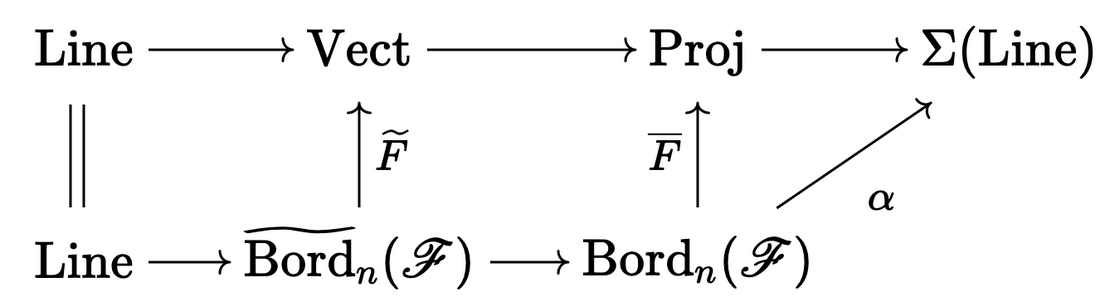
This is formally very much like the situation with groups. We even have a functor $\alpha$ which we interpret as an anomaly into a “shifted” category of $\text{Line}$. This $\Sigma(\text{Line})$ is a groupoid of gerbes (whatever that is). We also have $\overline{F}$ as a projective representation of the bordism category which we say is relative to $\alpha$. We can then ask about lifts of $\overline{F}$ to a functor $F$ into $\text{Vect}$. Being able to lift is, as before, equivalent to $\alpha$ being trivializable and “ratios” of trivializations correspond to invertible $n$-dim theories.

Sometimes, we also have that the $n$-dim theory extends to an $(n+1)$-theory which is to say that we an embedding $\text{Bord}_n(\mathscr{F}) \hookrightarrow \text{Bord}_{n+1}(\mathscr{F})$ and $\alpha$ extends to the $(n+1)$-dimension.

Differential Cohomology

Let $h$ be any cohomology theory for CW complexes but typically it will be singular cohomology or K-theory. Then, differential cohomology refines $h$ to $\check{h}$ on smooth manifolds. For example, 1st singular cohomology $H^1(M,\mathbb{Z})$ can be thought of as maps $\phi:M \to S^1$ up to homotopy while $\check{H}^1(M,\mathbb{Z})$ is just the maps, not up to homotopy. Or $H^2(M,\mathbb{Z})$ gives principal $S^1$-bundles up to isomorphism while $\check{H}^2(M,\mathbb{Z})$ gives $S^1$-connections on $S^1$-bundles up to isomorphism. This is viewed as a differential refinement.

We have a map $\check{H}^2(M,\mathbb{Z}) \to \Omega^2_{\text{closed}}(M)$ which is curvature and also a map to $H^2(M,\mathbb{Z})$ which is the Chern class.

There is some kind of discussion for generalized differential cocycles on bordisms like these maps that Freed has worked on with Mike Hopkins and Constantin Teleman. I didn’t understand this.

There is also another point which is if we have a fiber bundle of fields $\pi:\mathscr{F} \to \overline{\mathscr{F}}$ where the target are background fields and the fibers are fluctuating fields. You might want to “integrate” out the fibers some how. It seems that this “integrating” out is interpreted as quantization or put another way, as linearization. But the anomaly can obstruct quantizing.

Anomalies of a Spinor Field

Consider Minkowski spacetime and let $C \subset \mathbb{R}^{1,n-1}$ be time-like vectors with a positive time-orientation (so in some positive cone). We have a Lorentz spin group $\text{Spin}{1,n-1} \subset Cl{n-1,1}^0$ in a Clifford algebra.

The spinor field data that we need is a real ungraded $Cl_{n-1,1}^0$-module $\mathbb{S}$.

Fact: The Lorentz signature $(1,n-1)$ is the only signature such that inside of the spin representation $\mathbb{S}\times \mathbb{S}$, there sits a copy of the vector representation of the standard $Cl_{n-1,1}^0$ action on $\mathbb{R}^{1,n-1}$ (I’m confused as to why the indices switch like this).

Hence, we have a pairing $\Gamma:\mathbb{S}\times \mathbb{S} \to \mathbb{R}^{1,n-1}$ which is a symmetric $\text{Spin}_{1,n-1}$-invariant form and $\Gamma(s,s)$ is always contained in the closure of the positive time-like cone $C$. We can also ask for a pairing $m:\mathbb{S}\times \mathbb{S} \to \mathbb{R}$ which is like $\Gamma$ in terms of invariance but skew-symmetric. It is interpreted as mass.

Now, if $\mathbb{S}$ is irreducible, $\Gamma$ exists uniquely. We may then extend $\mathbb{S}$ to be a module over $Cl_{n-1,1}$ (not just the even part). I believe that all finite dimensional $Cl_{n-1,1}$-modules arise this way from irreducible spin representations (I recall this from studying Morgan’s Seiberg-Witten theory book).

Lemma (Freed-Hopkins): Nondegenerate mass terms for $\mathbb{S}$ are in 1-1 with $Cl_{n-1,2}$-module structures on $\mathbb{S}\oplus \mathbb{S}^*$ which extend the $Cl_{n-1,1}$-module structure.

For $(\mathbb{S},\Gamma,m=0)$, what is the anomaly? It comes from an $(n+1)$-dim theory which has some curvature built out of the $\widehat{A}$-genus. The lemma tells us that if the mass is nondegenerate then there is actually a trivial anomaly. The anomaly only depends on $\mathbb{S}$ up to other modules that extend to $Cl_{n-1,2}$-modules.

The interpretation of this is somehow related to Atiyah-Bott-Shapiro’s view that the abelian group of equivalence classes of $Cl_{n-1,1}$-modules modulo those that extend to $Cl_{n-1,2}$-modules in terms of the KO-theory spectrum. So $[\mathbb{S}] \in \pi_{2-n}(KO) \cong KO(pt)$. Then the anomaly is some lift of a map out of $M\text{Spin}$. One place to learn more about Clifford algebras, Dirac operators, and K-theory is Jiahao Hu’s very good thesis.