Basics of Linear Regression

These are notes I made while learning about the subject from my former colleague Victor Churchill’s lecture notes. Regression is a type of supervised learning that models the relationship between one or more independent variables (features) and a continuous dependent variable (target). The goal of regression is to predict the value of the dependent variable based on the values of the independent variables. The main example we look at here is linear regression.

Before we apply linear regression to data, we need to make the following assumptions about the data.

1. Linearity: the relationship between the feature set and target variable is linear
2. Homoscedasticity: the variance of the residuals (related to error $\epsilon$) is a constant $\sigma^2$.
3. Independence: all observations are independent of one another
4. Normality: the distribution for the error $\epsilon$ is normal $N(0,\sigma^2)$; the mean is assumed to be 0; so on average, we expect the error to be about equal measures of positive and negative values.

Remark: There may be many sources of error such as error in the measuring device, bias, etc. If we believe they are independent and we sum them up, the Lyapunov Central Limit Theorm tells us that these should compound together to give a normal distribution.

Caution: If the dataset does not have these properties, we should not use linear regression or at least be very cautious about making conclusions!

But supposing the dataset of $n$ points does have the properties, we work with a vector $\beta = (\beta_0,…,\beta_{p-1})$ of parameters and the inputs form an $n \times p$ design matrix $X$ (where the first column are all 1’s). Thus, we have $y=X\beta + \epsilon$, a vector of outputs with $\epsilon$ being error. For example, if $X$ is just a row vector, then $y =\beta_0 + \beta_1 x_1+…+\beta_{p-1}x_{p-1}$; we think of $\beta_0$ like a $y$-intercept.

We usually want to minimize the residual sum of squares $RSS = (y-X\beta)^\top(y-X\beta)$ which we can compute by considering the actual values of $y$ compared to the predicted values. One way to measure goodness of fit is $R^2 = 1-RSS/TSS \in (-\infty,1]$. The $RSS$ is the squared difference between the actual values and the predicted values (residual squared errors). On the other hand, $TSS$ is the squared difference between the actual values and their mean. Since $TSS$ stands for total squared errors, you might think $RSS$ is a percentage of this and hence, $RSS/TSS \in [0,1]$. But in fact, that’s not the case, we can have $RSS>TSS$ (so the model does worse than merely predicting the mean as a baseline) and hence, $RSS/TSS \in [0,\infty)$ and so $R^2 \in (-\infty,1]$; a model can be arbitrarily bad.

Note that if we simply predicted the average value of $y$, we’re not using any of the features from the data put into $X$. So a score $R^2 = 0$ means that our model isn’t finding anything useful about the features in $X$ and we may as well just be using the target data $y$. Thus, if $R^2>0$, we can interpret it as saying that the features in $X$ actually have some explanatory power for explaining why we observe $y$.

Now, if $y=\beta_0+\beta_1 x$ is only a model for a single variable, then $R \in [-1,1]$ is the correlation coefficient for $x$ and $y$. Squaring it will actually concide with the $R^2$ defined above; so in that case, there is a lower bound on $R^2$. And that’s why people named it $R^2$. But despite the name, with multiple linear regression, $R^2<0$ is possible! Also, by adding more features (making the model more complicated), we can increase $R^2$ but that doesn’t necessarily mean the model is getting better; we might just be overfitting the model on the training data. While I’m on this lengthy tangent, we can always do some scaling of predictors or add constants to them. We can even rescale the target $y$. However, it’s not hard to see that $R^2$ is invariant under these changes.

We can also measure how good of a fit the model is via MSE (mean squared error) which measures the variance of the residuals or the MAE (mean absolute error) which measures the average of the residuals. MSE penalizes larger errors than MAE, making it more sensitive to outliers.

First of all, why would we pick MSE? Since we assume the errors are normally distributed and also the samples are independent, we can then get a maximum likelihood function that is simply a product of many Gaussians. If we take the log of it, what comes out is just a quadratic form which equals mean squared error. So the assumptions of normality and independence naturally lead us to MSE.

The way to find $\hat{\beta}$ that minimizes MSE is actually very explicit. Write $L(\hat{\beta}) = |y-X\hat{\beta}|^2$ as the squared error (the $1/n$ is just a constant so we can leave it behind). The gradient of $L$ can be used to find directional derivatives. So if we take a small step $h$ (this is a vector), then $L(\hat{\beta}+h) = L(\hat{\beta})+\nabla L(\hat{\beta})\cdot h + o(h)$; we have 0th, 1st, and higher order terms.

The LHS is $|y-X(\hat{\beta}+h)|^2 =|y-X\hat{\beta}|^2-2(y-X\hat{\beta})\cdot Xh + |Xh|^2$. The first term is clearly just $L(\hat{\beta})$ and the third term is bounded because $|Xh| \leq C|h|$ where $C$ is the operator norm of $X$, in this case, the largest of its singular values (recall singular value decomposition). Thus, the middle term must be $\nabla L(\hat{\beta})\cdot h$. To put it in this form, a dot product can be rewritten as multiplication: $(y-X\hat{\beta})\cdot Xh = (Xh)^\top (y-X\hat{\beta}) = h^\top (X^\top (y-X\hat{\beta})) = X^\top(y-X\hat{\beta}) \cdot h$. Hence, $\nabla L(\hat{\beta}) = -2X^\top(y-X\hat{\beta})$.

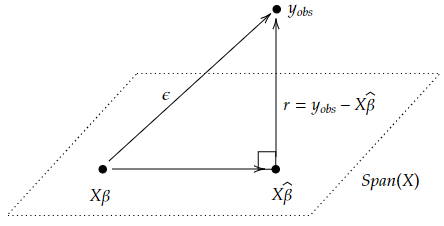
Now, we are looking for $\hat{\beta}$ so that this equals 0. By definition of adjoints, $\langle X^\top(y-X\hat{\beta}), v \rangle = \langle y-X\hat{\beta},Xv \rangle$. So if $X^\top(y-X\hat{\beta})=0$, then this means that $y-X\hat{\beta}$ is orthogonal to $\text{Im}(X)$. Since $X \hat{\beta}$ is in $\text{Im}(X)$, we can reinterpret the orthogonality as minimizing the distance between $y$ and the subspace $\text{Im}(X)$. Put a different way, we’re looking for $\hat{\beta}$ so that $X\hat{\beta}$ is the projection of $y$ onto $\text{Im}(X)$.

\(\begin{align*} -\frac{1}{2}\nabla L(\hat{\beta}) =& X^\top (\vec{y} - X \hat{\beta}) = 0\\ & X^\top \vec{y} - X^\top X \hat{\beta} = 0 \\ & X^\top X \hat{\beta} = X^\top y\\ & \hat{\beta} = (X^\top X)^{-1} X^\top y \end{align*}\) So we have found the unique minimizer of the loss function $L$ in terms of $X$ and $y$ which we know explicitly from the data.

We could also have derived this more quickly just from linear algebra. We want to minimize $|\vec{y}-X\hat{\beta}|^2$. We can view $X\hat{\beta}$ as being a vector which is a linear combination of the columns of $X$. So we begin our search for $\hat{\beta}$ by looking at all possible such linear combinations which is the column space of $X$, some subspace. The shortest distance between a vector $\vec{y}$ and a subspace is the length of a vector that emerges from and is orthogonal to the subspace and ends at $\vec{y}$. At this point, we reuse what we saw above. To be orthogonal means $0= \langle y-X\hat{\beta},Xv \rangle$ for all $v$. But this inner product is equal to $\langle X^\top(y-X\hat{\beta}), v \rangle$ by adjointness so we want $X^\top y - X^\top X\hat{\beta} = 0$. Solving for $\hat{\beta}$, we get the formula.

Let’s next define the covariance of a random vector to be $\text{Cov}(\vec{v}) =E[(\vec{v}-E[\vec{v}])(\vec{v}-E[\vec{v}])^\top]$. It may seem weird that the covariance of a vector is a square matrix but one reason to define it this way is because, if $\vec{w}$ is a fixed vector, then the expected value of the $\text{Var}(\vec{v}\cdot \vec{w})$ is $\vec{w}^\top \text{Cov}(\vec{v})\vec{w}$. In this way, the covariance of $\vec{v}$ is used to project points onto the span of $\vec{w}$ and then we measure the spread on that 1-dim subspace.

Theorem: $E[\hat{\beta}] = \beta$ where $\beta$ is supposed to give the “true” linear coefficients. Moreover, $\text{Cov}(\hat{\beta}) = \sigma^2 (X^\top X)^{-1}$.

Proof: Since $y = X\beta + \epsilon$, then $\hat{\beta} = (X^\top X)^{-1}X^\top y = (X^\top X)^{-1}X^\top (X\beta +\epsilon) = \beta + (X^\top X)^{-1}X^\top \epsilon$. Expected value is linear so $E[\hat{\beta}] = \beta + (X^\top X)^{-1}X^\top E[\epsilon] = \beta$. For the covariance, if $z = c+Ay$ where $y$ is random but $A,c$ are fixed, then $\text{Cov}(z) = A\text{Cov}(y)A^\top$. Applying this, where $c = \beta$, $A = (X^\top X)^{-1}X^\top$, we get the result.

Estimating $\sigma^2$

To find the covariance of $\hat{\beta}$, we need $\sigma^2$. Let’s try to estimate $\sigma^2$. We let $\hat{\epsilon} = y-\hat{y}$ be the residuals; i.e. the difference between the observed value and our predicted value. Anyways, $y-\hat{y} = y-X\hat{\beta} = y-X(X^\top X)^{-1}X^\top y = (I-P)y$ where we set $P=X(X^\top X)^{-1}X^\top$.

Remark: It looks like the definition of $P = X(X^\top X)^{-1}X^\top$ makes $P=I$ but remember, $X$ is not necessarily a square matrix and so it might not be invertible on its own. It’s only $X^\top X$ that we’re assuming to be invertible. That happens if and only if $X$ has full rank $p$.

This $P$ is an orthogonal projection matrix onto $\text{Im}(X)$. All projection matrices are idempotent which means $P^2=P$ and $P$ is also symmetric. For that reason, note that $I-P$ is also idempotent and symmetric. Moreover, the rank of $P$ is $p$; the eigenvalues of $P$ consist of $p$ ones and $n-p$ zeros. It’s also easy to see that $PX=X$.

Theorem: Given $n$ datapoints which each have $p-1$ independent features (remember, $\beta_0$ is not paired with an $x_0$), assuming the errors are uncorrelated with constant variance $\sigma^2$, an unbiased estimate of $\sigma^2$ is $s^2 = \dfrac{|y-\hat{y}|^2_2}{n-p}$.

The proof of this isn’t too hard. It utilizes the following useful lemma: If $\vec{x}$ is a random variable with mean $\vec{\mu}$ and covariance $\Sigma$ and $A$ is a fixed matrix, then $E[\vec{x}^\top A\vec{x}] = \text{tr}(A\Sigma) + \vec{\mu}^\top A\vec{\mu}$. Also, we see that it’s important to have more observations $n$ than features $p$.

Analyzing the Residual

It turns out that the residual (the difference between observed and predicted) $\hat{\epsilon}:= y-\hat{y} = (I-P)y$ contains information about how good the model fits. Lemma: $\text{Cov}(\hat{\epsilon}) = (I-P)^\top (\sigma^2 I)(I-P) = \sigma^2(I-P)$.

This relies on the lemma we mentioned above: For the covariance, if $z = c+Ay$ where $y$ is random but $A,c$ are fixed, then $\text{Cov}(z) = A\text{Cov}(y)A^\top$. Moreover, since $I-P$ is symmetric and idempotent, we get the final result.

Each coordinate of the residual $\hat{\epsilon} \in \mathbb{R}^n$ represents the residual for a single datapoint and there is correlation between residuals as we can read off from this covariance matrix. Also, different residuals have different variances, as we can read off from the diagonal of $I-P$. As such, we usually standardize them; the $i$th standardized residual is $\dfrac{\hat{\epsilon}}{s\sqrt{1-p_{ii}}}$ where $s$ is the unbiased estimate for $\sigma$ above.

Theorem: If the errors have covariance matrix $\sigma^2I$; i.e. they are have the same variance, then the residuals are uncorrelated with the fitted values; i.e. $\text{Cov}(\hat{\epsilon},\hat{y}) = 0$. Put another way, the residuals should look random.

Proof: If $y=Ax,z=Bx$ for fixed matrices $A,B$, then $\text{Cov}(y,z) = A\text{Cov}(x)B^\top$. In our case, $\hat{\epsilon} = (I-P)y, \hat{y} = Py$. So $\text{Cov}(\hat{\epsilon},\hat{y}) = (I-P)(\sigma^2I)P^\top = \sigma^2(I-P)P=0$. $\square$

Remark: Note that here, we didn’t need to assume that the errors are independent or normally distributed.

Inference on $\beta$

Now we will utilize our assumption that the errors are independent or normally distributed in order to make some inference on $\beta$; i.e. try to understand the underlying relationships between predictors and target via our coefficients. Recall that we had the following theorem from above:

Theorem: $E[\hat{\beta}] = \beta$ where $\beta$ is supposed to give the “true” linear coefficients. Moreover, $\text{Cov}(\hat{\beta}) = \sigma^2 (X^\top X)^{-1}$.

Also, since $\hat{\beta} = \beta + (X^\top X)^{-1}X^\top \epsilon$, $\hat{\beta}$ is a linear combination of independent, normally distributed random variables. Hence, $\hat{\beta}$ is also normally distributed (for proof, see here; remember that the PDF for a sum of random variables is not the sum of the PDFs but rather the convolution. For a proof of this second fact, see here). If $C = (X^\top X)^{-1}$, then $\hat{\beta}_i \sim N(\beta_i,\sigma^2 c_{ii})$.

Taking $s^2 = \dfrac{|y-\hat{y}|^2_2}{n-p}$ as above, the standard error of $\hat{\beta}_i$ can be estimated as $s_{\hat{\beta}_i}=s\sqrt{c_{ii}}$. We can then show that $\dfrac{\hat{\beta}_i-\beta_i}{s_{\hat{\beta}_i}} \sim t_{n-p}$ (the $t$-distribution is constructed from the normal distribution divided by a chi distribution with some scaling constant). As such, the $100(1-\alpha)$% confidence interval for $\beta_i$ is $\hat{\beta}_i \pm t_{n-p}(\alpha/2)s_{\hat{\beta}_i}$.

To run a hypothesis test, we can have $H_0:\beta_i = b$ for some fixed $b$ and use the test statistic $t=(\hat{\beta}_i-b)/s_{\hat{\beta}_i}$, then compute the p-value. Commonly we set $b=0$ to test whether the $i$th independent variable $x_i$ has predictive value.

More on Confidence Intervals for Linear Regression

We have some “true” relation $y=X^\top\beta + \epsilon$ for the total population where the error is normally distributed with variance $\sigma^2$ and $X \in \mathbb{R}^{p+1}$ with the first coordinate being 1. So if we wrote this out, we’ll see $y=\beta_0+\beta_1x_1+…+\beta_px_p$.

We can build a model that has some $\hat{\beta}$ to try and predict the true relation but we build it from samples so it will likely not be quite right. With a slight abuse of notation, let $X_0 \in \mathbb{R}^{p+1}$ as well with the first coordinate being 1. What is $X_0^\top \hat{\beta}$? It is a single value function and we obtain $\hat{\beta}=(X^\top X)^{-1}X^\top y_{obs}$. But $y_{obs}=X\beta+\epsilon$. So then $\hat{\beta}=\beta+ (X^\top X)^{-1}X^\top\epsilon$. Thus, because $\epsilon \sim N(0,\sigma^2I)$, then $\hat{\beta}$ is also normally distributed. Also, recall that $X^\top X$ is symmetric and usually positive definite in which case, it is invertible. Then $(X^\top X)^{-1}$ has a square root.

Lemma: If $Z \sim N(\mu,\Sigma)$ is normally distributed where $\Sigma$ is the covariant matrix and $A$ is any linear transformation, then applying it to $Z$, we have $AZ \sim N(A\mu,A\Sigma A^\top)$.

By the lemma, $\hat{\beta} \sim N(\beta,\sigma^2(X^\top X)^{-1})$. Applying $X^\top_0$ we have $X^\top_0 \hat{\beta}\sim N(X^\top_0 \beta,\sigma^2X^\top_0 (X^\top X)^{-1} X_0)$; this single-variable and we can see that the variance is back to just being a single number, not a matrix.

Lastly, $W=X^\top_0(\hat{\beta}-\beta)/\sigma\sqrt{X^\top_0 (X^\top X)^{-1} X_0} \sim N(0,1)$. Now, the thing in the numerator is the difference between the fitted models mean response and the true meal response. If we know $\sigma$ (the true standard deviation), we’ll be done now and can get the confidence intervals: $z_{\alpha/2} \leq X^\top_0(\hat{\beta}-\beta)/\sigma\sqrt{X^\top_0 (X^\top X)^{-1} X_0} \leq z_{1-\alpha/2}$.

Then rearranging, the long formula for the $(1-\alpha)$-confidence interval is: $X^\top_0\hat{\beta}-z_{1-\alpha/2}\sigma\sqrt{X^\top_0 (X^\top X)^{-1} X_0} \leq X^\top_0\beta \leq X^\top_0\hat{\beta}+z_{1-\alpha/2}\sigma\sqrt{X^\top_0 (X^\top X)^{-1} X_0}$.

But we don’t usually know $\sigma$! So we need to understand how $W$ is distributed. If we have replace $\sigma$ with the sample standard deviation $\hat{\sigma}$, then: $X^\top_0(\hat{\beta}-\beta)/\hat{\sigma}\sqrt{X^\top_0 (X^\top X)^{-1} X_0} = \frac{\sigma}{\hat{\sigma}}W = \left(\frac{\frac{1}{n-p-1}|X^\top_0\hat{\beta}-y_{obs}|^2}{\sigma^2}\right)^{-1/2}W$.

Claim: The thing with the parentheses and the $-1/2$ power can be viewed as the denominator while $W$ is viewed as the numerator. $W \sim N(0,1)$ (we already knew this) while the denominator has distribution $\chi^2_{n-p-1}/(n-p-1)$. moreover, the two are indepedent. Thus, by definition, the two together gives the $t$-distribution $T_{n-p-1}$ with $n-p-1$ degrees of freedom.

To prove independence, we can draw a picture.

We assume that $X$ has full-rank and so though it doesn’t have an inverse on its full codomain, it has one at least on its image (a left inverse) which we’ll just write as $X^{-1}$. Then the numerator of $W$ which is $X^\top_0\hat{\beta}-X^\top_0 \beta$ can be written $X^\top_0X^{-1}(X\hat{\beta}-X \beta)$. But $X\hat{\beta}-X \beta$ lies in $\text{Span}(X)$ while the residuals $y_{obs}-X\hat{\beta}$ lies in the orthogonal complement $\text{Span}(X)^\perp$. So those two are independent. Moreover, applying linear maps won’t change independence. Thus we’ve proven independence. Also, more or less by definition, we see that the denominator term is the $\chi^2$ distribution described above. Thus, the quotient above is the $t$-distribution, by definition.

Aside: The probability density function of the $t$-distribution is not the quotient of the PDFs of the other two. If it were, the $t$-distribution would not be symmetric but we know from other means that it should be.

With that said, we can then give a confidence interval when we don’t know the true variance $\sigma^2$.

Another aside: Above, I said that $(X^\top X)^{-1}$ has a square root; choose one and call it $R$. Then $\sqrt{X^\top_0R^TRX_0} = |RX_0|$ defines a metric called the Mahalanobis metric.

Collinearity and Overfitting

In Churchill’s notes, he shows some data of the heights and weights of children with heart defects as well as the length of catheters needed to reach their pulmonary artery for treatment. Assuming there’s some linear relationship between (height, weight) and catheter length, he ran a linear regression and then did two hypothesis tests where $H_0:\beta_i=0$ for $i=1,2$ since we have two features: height and weight. Interestingly, we find rather high p-values for both.

On the other hand, if you run two separate linear regressions, each one only taking into account one feature, then the hypothesis tests will reveal very low p-values whcih means we have significant findings: height is related to catheter length and weight is related to catheter length.

What is going on here? Clearly there is a linear relationship in the dependent variable, so why isn’t it showing up as significant when we regress using both features?

The answer is that the data exhibits collinearity. In our context, if we plot (height, weight, catheter length) in $\mathbb{R}^3$, we find that the data roughly lie on a single straight line rather than a plane. Collinearity means that the linear subspace spanned by the datapoints has dimension less than the number of features (remember, we’re assuming the data behaves linearly up to some error). Put another way, there’s some linear dependence.

This creates a problem for multiple regression. Recall the interpretation of the coefficients in a multiple regression. Holding all other $\beta_j$ with $j\neq i$ constant, the coefficient $\beta_i$ is the expected change in $y$ given a unit increase in $x_i$.

The key to the issue is with holding all other constant. Since the data is collinear, both the height and weight need to change together in order for the catheter length to change. If we hold height constant, a unit increase in weight will result in little change to the catheter length.

One way to address collinearity is to use principal component analysis or truncated singular value decomposition. What we can do is find the left and right singular vectors which will be orthonormal bases in the respective vector spaces. The singular values can be taken to be positive and ordered in decreasing order. Using the singular vectors (also called components), we have a new basis (so we no longer have linear dependence) and the singular values tell us how much those components contribute.

In the example, there are three components since the data are in $\mathbb{R}^3$ but one of components explains the relation far more than the other two. So we could do a regression where we end up with just one feature that is a linear combination of height and weight.

There are several metrics for determining the usefulness of a model. The coefficient of determination is $R^2 = \dfrac{s^2_y-s^2_{\hat{\epsilon}}}{s^2_y}$. This is the proportion of the sample variation in $y$ that is explained by the regression model (so the part that is unexplained is from the residuals).

We can also run a hypothesis test with $H_0:\beta_1=\beta_2=…=\beta_{p-1}=0$. The F-statistic $F = \dfrac{(s^2_y-s^2_{\hat{\epsilon}})/(p-1)}{s^2_y/(n-p)}$ is used for this hypothesis test.

Multiple linear regression can also be sensitive to outliers. For example, if we include a datapoint with the average height and weight but a very long catheter, this can shift the model quite a lot. This phenomenon is called overfitting. Here, the model is overly compensating the outlier when it would be better if the model ignored it or gave it less weight.

Regularization

One way to address overfitting is by regularization. We can include a penalty term in the loss function of linear regression. What it does is penalize $\beta$ with large norm (outliers would give larger $\beta$). Of course, this means we need to make a choice of norm.

In ridge regression, we want to solve a constrainted optimization problem: $\arg \min_\beta{|y-X\beta |^2_2}$ subject to $|\beta|^2_2 \leq c$ for some value $c$. This is equivalent to solving the following unconstrained optimization problem: $\arg \min_\beta {|y-X\beta|^2_2 +\lambda |\beta|^2_2 }$ for some value $\lambda$ called the regularizaion parameter.

Another way to think of regularization is from the perspective that we want to do a maximum likelihood estimate (MLE) for $\beta$ but we add in some prior belief about what that $\beta$ should be like. In this case, since we chose the $\ell^2$ norm, the distribution for our prior is Gaussian.

The least squares solution (which naturally comes out when doing MLE) is $\hat{\beta}_{ridge} = (X^\top X + \lambda I)^{-1}X^\top y$.

Another regularization is called LASSO: Least Absolute Shrinkage and Selection Operator. The only difference is that the norm we choose is $\ell^1$; then we can think of it as solving a constrained or unconstrained optimization problem like before. From a Bayesian view, the prior has a Laplace distribution.

LASSO has the feature of encouraging some of the components of $\beta$ to be zero.