Statistics Review

These are notes that I made when stuyding statistics from various sources, including the lecture notes of my former colleague Victor Churchill.

Remember: statistics is about using samples of a population to predict something about the entire population; e.g. given how these 100 students performed on the exam, how well did students across the nation do? Probability usually works the other way: you can know things about the whole population and you want to make predictions about samples; e.g. what’s the expected number of times you need to roll a 6-sided die in order to see a prime?

Just as brief reminder, given a probability space $(\Omega,\mu)$ and random variable $X:(\Omega,\mu) \to (\mathbb{R},dx)$, we can push forward the measure $\mu$. By Radon-Nikodym, if $X_*\mu$ is absolutely continuous with respect to the Lebesgue measure $dx$, then there exists a function $f$ called a probability density function and the pushfoward measure $X_*\mu((a,b)):=\mu(X^{-1}(a,b))$ can be computed by $\int^b_a f(x)\, dx$.

The expected value of a function $g$ is $E[g]=\int^\infty_{-\infty} g(x)f(x)\,dx$ and in particular, the expected value of the identity function $E[x]=\int^\infty_{-\infty}xf(x)\, dx$ is also just called the expected value of the random variable $X$. But we can also study the expected value of other functions. For example, the variance of a random variable $X$ is $\text{Var}(X) = E[(X-E[X])^2]=E[X^2]-E[X]^2$ which is always nonnegative. The latter is usually easier to compute. The standard deviaton $\sigma(X)$ is the square root of this.

We can also study conditional probability. The expectation of $X$ given $Y=y$ is $E[X|Y=y] = \int^\infty_{-\infty}xf_{X|Y}(x|y)\,dx$. Here, $f_{X|Y}$ is some other PDF.

If we have two random variables $X,Y$, the covariance is a linear measure of relationship between them, defined by $\text{Cov}(X,Y)=E[(X-E[X])(Y-E[Y])] = E[XY]-E[X]E[Y]$. The correlation is $\rho(X,Y)=\frac{\text{Cov}(X,Y)}{\sigma(X)\sigma(Y)}$. If we write this differently, we’ll see that the denominator is simply the geometric mean of the variances: $\sqrt{\text{Var}(X)\text{Var}(Y)}$. With this normalization, $\rho \in [-1,1]$. If $\rho>0$, we say $X$ and $Y$ are positively correlated; i.e. on the whole, as $X$ increases, so does $Y$. If $\rho<0$, they are negatively correlated and on the whole, as $X$ increases, $Y$ decreases. Note that the larger $|\rho|$, the stronger the correlation. So $\rho=0$ means there is no correlation and hence, $X$ and $Y$ are independent of each other. Put another way, $X$ and $Y$ are independent if and only if $E[XY]=E[X]E[Y]$. In the case that $X=Y$, we have $\text{Cov}(X,X)=\text{Var}(X)$ and $\rho=1$. Of course, $X$ should be perfectly correlated with itself.

Also, if we have $n$ identically and independently distributed variables $X_1,…,X_n$ and $\bar{X}=\frac{1}{n}(X_1+…+X_n)$, then $\text{Cov}(X_i-\bar{X},X_j-\bar{X})=0$ and $\text{Var}(\bar{X})=\sigma^2/n$.

Hypothesis Testing

A statistic is a function $F$ on $X$; since $X$ is a random variable (which is a function), then so is $F$. But for example, we can have $F(X_1,…,X_n):\Omega^n \to \mathbb{R}^n \to \mathbb{R}$ where the $X_i$ are all independently and identically distributed and $F(X_1,…,X_n)=(X_1+…+X_n)/n$ is the average.

A null hypothesis can really be any statement in probability. For example, it can be that “ $A$ and $B$ are correlated” but we can also have “ $A$’s mean is equal to $B$’s mean”, “$X$ has probability distribution function being a normal distribution”, or “the sequential data we received are picked randomly from an independently and identically distributed (iid) sample.” The idea is to assume that the null hypothesis is true; with the assumption plus a statistic $F$, we’re able to built a null distribution to study. We want to know that under our assumption, what is the probability that we get the real data that’s in front of us? For example, if we hypothesize that a coin has equal probability flipping heads or tails but in 1000 flips, we have only 10 heads, then our hypothesis seems very likely to be wrong. And so we’d want to reject it. Here’s the general procedure.

Procedure:

1. Define a null hypothesis $H_0$ and an alternative hypotheses $H_a$.
2. Define a test statistic $F$ to get a corresponding $p$-value. Typically, we determine $F$ by having collected some data. If we’re dealing with a continuous random variable, then the $p$-value is the probability of observing $F$ or anything more extreme than $F$. If it’s a discrete variable, then the $p$-value is the probability of observing $F$.
3. Choose a significance level $\alpha$ and use it to determine a “rejection region.” If the $p$-value falls into that region, then we reject the null hypothesis $H_0$. Otherwise we fail to reject $H_0$ which means that we might accept $H_a$ or just find the whole thing inconclusive.

To clarify (2), a test statistic $F$ needs to have its own assumed probability distribution in order for us calculate a $p$-value; remember, a $p$-value is a probability. Since $F$ takes in some random variables and gives real numbers as output, we can think of it as itself being a random variable and hence, we can interchangeably think of it as defining its own probability distribution. We’ll say more about this below. For example, say that $F$ is the sample mean of math SAT scores from 2024. Say in past years, the mean score is 590. We hypothesize the mean score for 2024 to be 590 as well. But from a sample of 100 students, we find the mean to be $F=640$. Then the $p$-value is the probability $P(F \geq 640)$ of observing the sample to mean to be at least 640, assuming that the true mean is 590. For this sample, we’ll assume that the distribution for $F$ is a normal distribution $N(590,\sigma/\sqrt{100})$. Then we can calculate the probability of observing at least 640 to be $(640-590)/(\sigma/10) = 500/\sigma$. Fist, note that in order for us to do this, we need to know $\sigma$ for the entire population of students that took the SAT in 2024, not just the 100 students. But even if it’s something wildly big like $\sigma=100$, in that case, observing 640 is 5 standard deviations from the mean and the chances of that is extremely low. The empirical rule says that for a normal distribution, the probability of observing something within one $\sigma$ is 68%; within two $\sigma$ is 95%, within three $\sigma$ is 99.7%. Seeing something within five $\sigma$ has probability 0.9999999999985. So to see something outside of five $\sigma$ has an extremely small chance; that would be our $p$-value. However, in our hypothesis testing, we also need to pick a significance level $\alpha$ to compare to. If we chose $\alpha$ to be even smaller than this value, then we would fail to reject the null hypothesis. However, much of the time, $\alpha = 0.05$ is chosen (somewhat arbitrarily). This choice can change depending on context; say in the medical field, they might be stricter and choose $0.01$. But anyways, certainly for $\alpha=0.05$, our $p$-value is smaller, so we reject the hypothesis that the true mean for 2024 is 590.

Note that in the procedure, we don’t actually need $H_a$ so long as we have a rejection region. The reason $H_a$ appears is that often in context, there is some direction we hope to go in. For example, a pharmaceutical company might develop a new drug. The previous drug was effective for 6 out of 10 people and the company hopes the new drug is an improvement on the proportion $p=0.6$. So the null hypothesis might be $H_0: p=0.6$ and the alternative is $H_a:p>0.6$. This would then lead us to use a 1-tailed test. But in other situations, like the SAT scores, we might not have any reason to believe the average score will be higher or lower than 590. Then $H_a:\mu \neq 590$ is used and we’d need a 2-tailed test.

Hypothesis testing is the basis for A/B testing where you have a control group A and an experimental group B. For example, maybe a company wants to known if email campaigns boost their sales and so there is a control group A which does not receive emails while group B does. The null hypothesis is that there is no difference in sales between the groups. The company hopes that they can reject this null hypothesis to justify all the money they put into email campaigns.

Definition: For any population parameter $\theta$, we can form a distribution for the corresponding estimator $\hat{\theta}$ that we get from taking samples. The distribution has an expected value $\mu_{\hat{\theta}}$ and we say that $\hat{\theta}$ is unbiased if $\mu_{\hat{\theta}}=\theta$.

Examples: Both the sample mean $\bar{x}$ and sample proportion $\hat{p}$ are unbiased estimators. The sample variance $\hat{\sigma}^2$ is a biased estimator when we take $\frac{1}{n}\sum^n(x_i-\bar{x})^2$ but if we use $\frac{1}{n-1}$ as a coefficient instead, it becomes unbiased; see below for Bessel’s correction.

Definition: An estimator $\hat{\theta}$ is consistent if, as the number of samples $n \to \infty$, the sequence of estimator sampling distributions converges (in measure) towards the true parameters value. This means they converge to a Dirac delta type of distribution concentrated on $\theta$.

Example: Both the corrected and uncorrected sample variances are consistent since, as $n \to \infty$, $\frac{n-1}{n} \to 1$. If we have iid samples $x_1,…x_n$, then $\bar{x}=(x_1+…+x_n)/n$ is consistent; the Central Limit Theorem tells us that the variance is $\sigma^2/n \to 0$ as $n \to \infty$. So the bell curves concentrate and degenerate to a Dirac delta distribution. We could also take $x_n$ and since it’s just a copy of the original random variable, it’s expected value is just the expected value of the original; call this $\mu$. Then $x_n$ is an unbiased estimator but it is not consistent because as $n \to \infty$, every distribution in the sequence is the same and does not converge to a Dirac delta distribution supported on $\mu$.

Some Common Test Statistics

$Z$-test: We assume that the sample size $n$ is large enough to invoke the Central Limit Theorem and that we know the variance $\sigma^2$ for the total population. Note that this is a pretty big assumption to make! Supposing our null hypothesis is that the mean is $\mu_0$, the $Z$-test for population mean is the quantity $z=\frac{\bar{x}-\mu_0}{\sigma/\sqrt{n}}$ lying on athe standard normal distribution $N(0,1)$. We would then find the probability of seeing this result or something more extreme; that is our $p$-value. Lastly, compare it to a chosen significance level $\alpha$.

$t$-test: This test is structured similarly to the $Z$-test but crucially, we use it when we have a smaller sample size $n$ and we do not know the population variance $\sigma^2$. Instead, we’ll use the sample variance $s^2$. This test requires us to take into account the degrees of freedom which, here, is just $n-1$ (for multiple regression this changes). Thus, to compute the sample variance, we also divide by $n-1$, not by $n$; this is important! $s^2 = \frac{1}{n-1}\sum^n_{i=1} (x_i-\bar{x})^2$. The $t$-test is then the quantity $t=\frac{\bar{x}-\mu_0}{s/\sqrt{n}}$, lying on a distribution that looks similar to a normal distribution but it has larger tails; i.e. extreme events happen with greater frequency.

$\chi^2$-test: there are a few versions of this test.

1. For variance: the null hypothesis says the population has some variance and this test is to determine whether we reject the hypothesis.
2. For independence: we can also test whether two variables are correlated or not.
3. For “goodness” of fit of a curve: we usually say a curve is a good fit if the sum of squared errors is low. The test statistic in this case is $\chi^2=\sum_i (O_i-E_i)^2/E_i$ where $O_i$ is the value we observed from data while $E_i$ is the expected/predicted value based on our curve model.

$F$-test (“analysis of variance”=ANOVA): This is used to test whether grouping categorically is meaningful. For example, we might group test takers by left or right-handedness. If the test scores between the two groups is very similar, then we’d probably conclude it’s not meaningful to make the distinction.

Wikipedia has a list of some other common test statistics.

Confidence Intervals

Above, we discussed a significance level $\alpha$ to which we compared our $p$-value. We can also construct so-called confidence intervals with a chosen $\alpha$. For example, if we’re studying sample means with $\alpha=0.05$, then $(1-\alpha)=0.95$ and we can build a 95% confidence interval. This is a range of values that, if we have a large sample, then the true mean lies inside of the range of values 95% of the time. For the $Z$-test, we assume that the distribution is approximately normal when we have a large number of samples and that its mean $\mu_{\bar{x}} = E[\bar{X}] = \bar{X}$ is equal to the true mean $\mu$. So we build the interval as $[\bar{x}-z_{\alpha/2}\frac{\sigma}{\sqrt{n}},\bar{x}+z_{\alpha/2}\frac{\sigma}{\sqrt{n}}]$. Here, $\sigma_{\bar{x}} = \sigma/\sqrt{n}$ and $\sigma$ is the true population standard deviation. To get this $z_{\alpha/2}$, we look for a $z$-score $z^*$ so that the area under the standard normal curve on the interval $[-z^*,z^*]$ is $(1-\alpha)$, our desired confidence level. For example, if $\alpha=0.05$, we want $0.95 = P(\mu_{\bar{x}} − z^* \sigma_{\bar{x}} < x < \mu_{\bar{x}} + z^*\sigma_{\bar{x}})$ $= P(−z^∗ < z < z^∗)$ $\Rightarrow 0.975 = P(z < z^∗)$ $\Rightarrow z^∗ = 1.96$.

However, we must be careful about our assumptions. The distribution is assumed to be approximately normal and the samples are independent. But it could certainly be the case that the true mean $\mu \neq \mu_{\bar{x}}$ and that it doesn’t lie within our confidence interval at all. We’re only saying that given the data that we have, we expect that if we conduct the experiment 100 times and construct 100 confidence intervals, the true mean would lie in 95 of those confidence intervals. We’re not saying there’s $100(1-\alpha)$% chance that $\mu$ lies in a given interval because it’s a fixed number, not a random variable. It’s important to be careful; confidence intervals are often misinterpreted.

Now, in the example above, we are assuming we know $\sigma/\sqrt{n}$ but in practice, we don’t know the true population parameter $\sigma$. We only know $s/\sqrt{n}$, the sample standard deviation divided by $\sqrt{n}$. We can try to approximate $\sigma/\sqrt{n}$ with $s/\sqrt{n}$ but this generally works better only if $n$ is large. In such a scenario, we have to use a $t$-distribution which has a similar shape of density function as a normal distribution but it is algebraic (unlike $e^{-z^2/2}$ which is not) and has larger tails so that extreme events are more common. In particular, $t$-distributions are not weighted sums of normal distributions. This is because the sum of normal random variables is still normal. On the other hand, a $t$-distribution depends on a parameter called degrees of freedom $df = n-1$ which is, in this case, just one less than the number of samples and is related to why $s$ has a factor of $1/(n-1)$ instead of $1/n$ to make it an unbiased indicator.

Anyways, we’re able to get a $t$-score to build a confidence interval $\bar{x} \pm t^* \frac{s}{\sqrt{n}}$. Thus, for small $n$, we use this recipe instead of the one from earlier. Note that if we know that we’re sampling from a normal distribution $X$, then $\bar{X}$ is automatically a normal distribution as well. However, if we don’t know $\sigma$, then may still need to use $s$ if $n$ is small and thus, also use $t^*$ instead of $z^*$.

One technique for trying to estimate the sampling distribution is to just repeatedly draw samples with replacement from our observed data. So if we have 30 data points, we can do this resampling thousands of times. This technique is called bootstrapping. Note that it won’t improve our accuracy for estimating population parameters since it’s still the same 30 points, it’s only meant to give us a sense of the sampling distribution. However, from this bootstrapping, we’re able to build confidence intervals.

Below when discussing the $\chi^2$ distribution and maximum likelihood estimator, we’ll see some more confidence intervals.

Sample distributions with a large number $n$ of samples

The central limit theorem tells us that for any distribution, if we make $n$ iid samples, then the distribution for the sample average converges to a normal distribution as $n$ gets large. Moreover, the variance of that normal distribution is $\sigma^2/n$ where $\sigma^2$ is the variance of the original population. One thing to note is that when we perform samples in real life situations, we are almost never actually taking independent samples because we do so without replacement. For example, if we put out a survey, we don’t want the same person to fill out the survey multiple times. Now, if we take lots of random surveys from a large population, this hardly matters. But if we have a small population and we sample without replacement, we might still have convergence to a normal distribution but the variance might not be the predicted $\sigma^2/n$.

Anyways, let’s move on since there are other test statistics other than taking the average. What happens for these?

Let’s focus on proportion; there is also $t$-distributions which are similar to normal distributions but with larger tails. Recall that for a binomial distribution with probability $p$ of a single success and $1-p$ for failure, the chance of $k$ successes out of $n$ is ${n\choose k} p^k(1-p)^{n-k}$. The expected value is $\mu=np$ and $\sigma^2 = np(1-p)$.

Suppose we now want to sample the population to find some proportion. For example, the proportion of people who voted for the Democratic presidential ticket in 2016 to the total population (it was 0.48 for Hillary, 0.45 for Trump, some voted for other candidates).

We can sample $n$ people and ask how they voted (assume they’re truthful). So the proportion $\hat{p}=X/n$ where $X$ is the number of successes out of the total. The expected value $E[X/n]=\frac{1}{n}E[X] = \frac{1}{n}\cdot np$ (integration is linear). So $\mu_{\hat{p}}=p$. On the other hand, to find the variance, if we multiply a random variable by a constant $c$, then $\text{Var}(cX) = c^2\text{Var}(X)$ (easily seen from the definition). The variance here is $\frac{1}{n^2}\cdot np(1-p)$ and hence, $\sigma_{\hat{p}} = \sqrt{\frac{p(1-p)}{n}}$ which is equal to the original standard deviation divided by $n$. This is different than for the sample mean. For the sample mean distribution $\bar{x}$, $\mu_{\bar{x}}=\mu$ (mean equals the “true mean”) but $\sigma_{\bar{x}}=\sigma/\sqrt{n}$ which we know from the Central Limit Theorem. So the formulas are a bit different between $\hat{p}$ and $\bar{x}$.

Type I and Type II Errors

Type I (false positive): rejecting the null hypothesis when it’s correct. The value we would consider here is $1-\alpha$, the confidence level. Remember that we when our $p$-value is less than $\alpha$, that’s when we reject $H_0$. So $\alpha$ is the likelihood of us rejecting $H_0$ when it is in fact, correct.

Type II (false negative): failing to reject the null hypothesis when it’s incorrect The value to consider here is $1-\beta$, the power. This $\beta$ is the likelihood of failing to reject $H_0$ when it is incorrect. One way to set this up is to assume the alternative hypothesis $H_a$ is true and then rejecting $H_a$ (thereby, failing to reject $H_0$) as we’ll see in the example below. If we plot sample size vs. power, generally we see that more samples lead to a larger power. Usually we want $\alpha,\beta$ both to be small. However, we cannot usually make both small simultaneously.

Example: The average height for a European adult man is 178 cm with a standard deviation of 9 cm. Thus, if $x$ is defined as the random variable representing a given European man’s height, the distribution for $x$ is approximately normal with mean $μ = 178$ and standard deviation $\sigma=9$. However, in a survey of 64 adult Czech men, the average height was found to be 181 cm. Question: Are Czech men really taller than normal, or was this this just an artifact of the sampling?

Let $\mu$ denote the “true mean” for the height of Czech men and do a 1-sided test. We have $H_0:\mu \leq 178, H_a: \mu>178$.

We’ll assume $n=64$ samples is large enough to give us that $\bar{x}$ is a normal distribution $N(178,9/\sqrt{64})$. Note that the mean is 178 because for our null hypothesis, we’re assuming average Czech men are not taller than average European men. Then, assuming that 181 cm came from this distribution, we see that its $z$-score is $(181-178)/(9/8) =8/3 \approx 2.67$. We now need a rejection region. If we choose $\alpha =0.05$, our rejection is $z>z^*$ where $P(z>z^*))=\alpha$. In this case, $z^*\approx1.65$. Since our $z$-score of $2.67 >1.65$, we reject $H_0$. We can be more specific and get a $p$-value which is $P(z > 2.67) \approx 0.0038< 0.05$. This gives a particular quantity that tells us it’s very unlikely to see the results we did from the 64 Czech men and for them to be, on average, no taller than the average European man.

If our $H_0:\mu=178$ and $H_a:\mu \neq 178$, we’d have needed a 2-tailed test and our rejection region would have been in two pieces $|z|>z^*$. In that case, with $\alpha=0.05$, then $z^*\approx 1.96$ but even then, $2.67>1.96$. The $p$-value would be $P(|z| > 2.67)= 0.0076<0.05$. So we still reject.

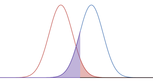
Now, in the 1-tail test example, we had a $z$-score of 1.65 given to us by having chosen $\alpha=0.05$. So we use the value $\bar{x}_0=178 + 1.65(9/8)\approx 179.856\, \text{cm}$; this is the cutoff in our rejection region. If the average height of the Czech men had been 179, we would not reject our original $H_0$. So now, to try and determine the likelihood of failing to reject $H_0$ when it is in fact correct, let’s set up a new hypothesis test where we let $H_a:\mu = 181$; we have many choices for the value here but we pick 181 since it’s the average height of the 64 sampled Czech men. Specifically, we set $\mu_a = 181$ but keep the same standard deviation. So this simply translates the normal distribution.

Finally, $\beta$ is the likelihood of accepting $H_0$ (which means rejecting $H_a$), i.e. the area under the curve to the left of $\bar{x}_0$ in the new distribution $N(\mu_a, \sigma_{\bar{x}})$ (the area to the right defined our reject $H_0$ region). So we see that if the area to the right is small, the area to the left will be usually be large even after adjusting $\mu_a=181$. This is why we’re not usually able to simultaneously make $\alpha$ and $\beta$ as small as we want. To calculate $\beta$, we find a new $z$-score: $z^∗_a =(\bar{x}_0 -\mu_a)/\sigma_{\bar{x}}$ and calculate $\beta := P(z < z^∗_a)$. In our situation, we have $z^∗_a= (179.856−181)/(9/8) \approx -1.02$. So $\beta = P(z < −1.02) = 0.1539$ is the likelihood of accepting $H_0$ when it is in fact, incorrect.

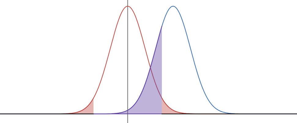
Here are two distributions. The red one is associated to $H_0$ with $\mu = 178$ and the blue one for $H_a$ when we choose $\mu_a=181$; so it’s simply the red curve shifted to the right. The shaded red area is $\alpha=0.05$ and the shaded blue region is $\beta=0.1539$. Note that I’m using the same $x=179.856 \text{ cm}$ to define the boundaries of the red and blue regions. It’s a bit hard to see but the black line on the $x$-axis is the rejection region. So to compute $\beta$, we need to look at the area under the new distribution assuming $\mu_a$, over the complement of the rejection region.

Remark: In general, $\alpha+\beta \neq 1$. We can do whatever we like in setting $\mu_a$ and it will not affect $\alpha$. In this way, we’re able to make $\beta$ whatever we like; e.g. make $\mu_a$ really big. However, if we’re trying to be honest about the power of our statistical test, we should pick a reasonable $\mu_a$. For example, it’s dishonest to pick 300 cm since that’s saying we hypothesize that Czech men are 3 meters tall.

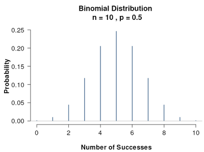
Example: Consider a simpler situation. Suppose we flip a possibly biased coin 10 times and see 9 tails. We can do a hypothesis test as follows. Let $H_0:p=1/2$ where $p$ is the probability of getting heads. We choose $1/2$ since the coins we’re used to are fair. And $H_a: p<1/2$. The probability of seeing 9 or more tails out of 10 flips if $p=1/2$ is the same as seeing 1 or fewer heads out of 10: ${10 \choose 0}(1/2)^{10}+ {10 \choose 1}(1/2)^1(1/2)^9 = 11/1024 \approx 0.010$. If $\alpha =0.05$, then this $p$-value is $P(N\leq 1) <\alpha$ and so we’d reject the null hypothesis. However, $P(N \leq 2) \approx 0.0546>\alpha$. So the rejection region is defined by $N=0,1$ heads.

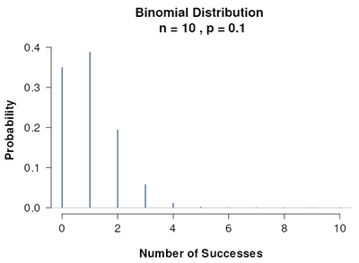
Now, based on this accept/reject method, we want to compute $\beta$; i.e. the probability of type II error which is accepting $H_0$ under another concrete assumption. Earlier, that assumption was $\mu_a=181$. Here, let’s set the assumption to be that $p = 1/10$ since we saw only one heads out of 10 flips. So we get a new distribution.

Under this new assumption $p=1/10$, the probability of our rejection region is the sum of the following: $P(N=0) = (9/10)^{10} \approx 0.3486$ $P(N=1) = {10 \choose 1} (1/10)^1 (9/10)^9 \approx 0.387$.

Hence $\beta=P(\text{accept } H_0) = P(N\geq2)= 1-P(N=0)-P(N=1) \approx 0.2644$.

There is a online widget for visualizing binomial distributions. The first one is when $p=1/2$, the second when $p=1/10$.

Remark 1: $\beta$ not only depends on an extra concrete assumption (in this discrete case $p=1/10$, in the previous case $\mu_a=181$), it actually depends on the rejection region we computed in the first step.

Remark 2: We can also conduct two tailed tests like this one where the rejection region is in two pieces. However, the complement of the rejection region is in one piece hence, there’s only one shaded blue region.

Maximum Likelihood Estimation in the Discrete Setting

Example: Suppose we have a biased coin with probability $p$ of getting H. We toss the coin 80 times and it comes up heads 49 times. The probability of seeing this is $L(p)={80 \choose 49}p^{49}(1-p)^{31}$. That is, $L(p)=P(\text{Data}|p)$, a conditional probability for any fixed $p$. But we’re going to let $p$ vary and so for each $p$, we do get a different probability distribution.

Note this is a polynomial where the leading term is $-{80 \choose 49}p^{80}$; this is negative so if we find a unique local max, it will in fact be the global max. To find the maximum of $L$, we can differentiate: $\frac{dL}{dp}={89\choose 40}(49 p^{48}(1-p)^{31} -31p^{49}(1-p)^{30}) = {89\choose 40} p^{48}(1-p)^{30}(49(1-p)-31p)$. Setting equal to zero, we have solutions when $p=0,\frac{49}{80},1$. But $F$ is minimized (equals 0) when $p=0,1$ and is maximized at $49/80$. Thus the most likely value of $p$ given this experiment is $49/80$. That’s exactly what we would expect.

Remark: Our function $L$ is used for determining the likelihood, hence the choise of letter. Also, it’s not important to have the constant ${80 \choose 49}$ in front to learn the maximum. But also, the function $\log$ is monotonically increasing (and convex) and so the critical points of $L$ and $\log L$ are the same. Here, it’s easier to work with $\log F = 49 \log p +31 \log(1-p)$ since multiplication is converted to addition. The derivative is $\frac{49}{p}-\frac{31}{1-p}$. Setting this to zero and doing some cross multiplication: $49(1-p)-31p=0$ so then $p=49/80$.

But now, change the situation a bit. Suppose we know that this biased coin can have only one of three values for $p$: $1/3, 1/2, 2/3$. We flip the coin 80 times and get 49 heads. If we plug these values into our function $L$ from above, we’ll find $L(2/3)$ is the largest and thus, $p=2/3$ is the most likely for our coin, given the experimental results.

In the literature, people often use $\theta$ as the symbol instead of $p$ so let’s use that in the sequel.

Remark: Another reason to take the logarithm is that for computing, note that $p^{48}$ is very small when $p \in (0,1)$. We’ll have long floating point values. However, $\log(p^{48}) = 48\log(p)$ whose absolute value is larger than $p^{48}$ and so we’ll not have to work with as bad of floats.

Maximum A Posteriori in the Discrete Setting

Now usually, real world coins have $\theta \approx \frac{1}{2}$. In the situation above we are told that the coin (might be) biased, and so it is reasonable to guess that $\theta= \frac{4}{5}$ if you observe $4$ heads and $1$ tail out of 5 flips, say. Without being given any such information, we might instead think that the distribution of weights could look something like $P(\theta) = k \theta^8 (1-\theta)^8$ where the constant $k$ has been chosen to make the integral equal to $1$ over $[0,1]$ (it turns out that $k = \frac{1}{B(9,9)}$ where $B$ is the “beta” function. See beta distribution for more info). This $P(\theta)$ is the prior which is based on our prior experience that coins are usually fair.

Assume that we flip our coin $5$ times and obtain $4$ heads as before but we also know that “normal” coins have $\theta=1/2$ and prior to flipping we thought to ourselves “If I flip this coin 16 times, I expect 8 heads.” So instead of estimating $\theta = 4/5$ we should now guess something in between $4/5$ and $1/2$. How can we calculate it exactly? Bayes Rule is useful: $P(\theta | \textrm{Data})\propto P(\textrm{Data}| \theta) \cdot P(\theta)$ $\propto \theta^4(1-\theta)^1 \cdot \theta^8(1-\theta)^8$ $\propto \theta^{4+8}(1-\theta)^{1+8}$ $= \theta^{12} (1 - \theta)^9$

We have maximized this type of thing before: the maximum value occurs at $\hat{\theta} = \frac{12}{21} = \frac{4}{7}$.

Note that $P(\theta | \textrm{Data})$ is the “posterior probability”. We are maximizing this term, hence maximum a posteriori estimation. To summarize the terminology:

Since $P(\text{Data})$ is constant with respect to $\theta$, we don’t need to worry about it much. Our prior can be interpreted as being equivalent to 16 “pseudo-observations” with 8 heads and 8 tails. Intuitively you could say something like “Since most coins I have seen are balanced with $\theta=1/2$, I will give this coin a ‘head start’ of 8 heads and 8 tails before estimating my parameter $\theta$. This is to incorporate my belief that coins are usually weighed fairly.” If I’m very confident, I might decide to give the coin a headstart of 100 heads and 100 tails and it’s going to take a lot of coin flips to convince me that $\theta$ is far from $1/2$.

Note that if $P(\theta)$ is also constant like it would be in a uniform distribution, then $P(\theta|\text{Data}) = C \cdot P(\text{Data}|\theta)$; i.e. just constant multiples of each other. This means that up to a constant, MLE is equivalent to MAP with a uniform prior distribution. In terms of pseudo-observations, we give it zero head start.

MLE in the Continuous Setting

Assume now that $n$ samples $x_1, x_2, x_3, \dots , x_n$ are drawn from a normal distribution with (unknown) mean $\mu$ and (unknown) variance $\sigma^2$.

We want to find figure out what are the most likely values for $\mu$ and $\sigma$, given our $n$ samples (think about the discrete situation). The more technical term is we’re looking for the maximum likelihood estimates $\hat{\mu}$ and $\hat{\sigma}^2$ of these parameters.

We want to maximize $L(\mu, \sigma) = \prod_{i=1}^{n} \frac{1}{\sqrt{2\pi} \sigma} \exp\left(-\frac{(x_i-\mu)^2}{2\sigma^2}\right)$.

Again, it is more convenient to turn this product into a sum using the logarithm. This is the log likelihood: $LL(\mu, \sigma) = \log\left( \frac{1}{\sqrt{2\pi} \sigma} \exp\left(-\frac{(x_i-\mu)^2}{2\sigma^2}\right) \right)$.

After a little algebra we have $LL(\mu, \sigma) = -n \log{\sqrt{2\pi}} - n\log(\sigma) - \sum_{i=1}^{n} \frac{(x_i-\mu)^2}{2\sigma^2}$.

This is a lot of minus signs, so we can instead think about minimizing the negative log likelihood: $NLL(\mu, \sigma) = n \log{\sqrt{2\pi}} + n\log(\sigma) + \sum_{i=1}^{n} \frac{(x_i-\mu)^2}{2\sigma^2}$. For ease of notation, call this $\ell$.

Its partial derivatives are:

Setting both equal to $0$ and solving, we obtain what we naturally would guess the mean and variance to be:

Bessel’s Correction

One mystifying thing is that when dealing with sample variance (rather than population variance), we often use the formula

which differs from the MLE estimate we just saw above, by a factor of $\frac{n}{n-1}$. This one with the $n-1$ is unbiased. while the one where we divide by $n$, it is biased. Why is that? Right away, we can see that in both formulas, we’re approximating the true mean $\mu$ by $\bar{x}$. So we should already expect to see some error due to this approximation.

Example

Let’s first consider an example. Suppose I have a discrete random variable that takes values $1,…,N$ with uniform probability. Then the mean is $E[k]=\sum^N_{k=1} k p(k)=(N+1)/2$. The variance is $E[(k-\mu)^2] = E[k^2]-\mu^2$. The sum of squares from 1 to $N$ is $N(N+1)(2N+1)/6$ and so the variance is $\frac{N^2-1}{12}$.

On the other hand, suppose we consider a random variable built from taking $n=2$ samples from here. So there are $N^2$ possible pairs $(1,1),(1,2),…,(N,N)$ each occuring with probability $1/N^2$.

Let’s just set $N=3$. So $\mu = (3-1)/2=2$ and $\sigma^2 = 8/12 = 2/3$.

Then sampling pairs, we have 9 pairs:

$\text{Pair} \hspace{16mm} \bar{x} \hspace{20mm} s^2$

$(1,1)\hspace{15mm} 1 \hspace{20mm} 0$

$(1,2)\hspace{15mm} 1.5 \hspace{15mm} 0.25$

$(1,3)\hspace{15mm} 2 \hspace{20mm} 1$

$(2,1)\hspace{15mm} 1.5 \hspace{15mm} 0.25$

$(2,2)\hspace{15mm} 2 \hspace{20mm} 0$

$(2,3)\hspace{15mm} 2.5 \hspace{15mm} 0.25$

$(3,1)\hspace{15mm} 2 \hspace{20mm} 1$

$(3,2)\hspace{15mm} 2.5 \hspace{15mm} 0.25$

$(3,3)\hspace{15mm} 3 \hspace{20mm} 0$

We have that $\bar{x}$ is a random variable which takes on values with probability:

$\text{Value} \hspace{10mm} p$

$1 \hspace{15mm} 1/9$

$1.5 \hspace{12mm} 2/9$

$2 \hspace{15mm} 3/9$

$2.5 \hspace{12mm} 2/9$

$3 \hspace{15mm} 1/9$

Note that the expected value of $\bar{x}$ is $\mu_{\bar{x}} = \frac{1}{9}(1*1 + 1.5*2+2*3+2.5*2+3*1) = 2$ which is the expected value of the original random variable. This shows our $\bar{x}$ is an unbiased estimator.

$s^2$ is also a random variable:

$\text{Value} \hspace{10mm} p$

$0 \hspace{15mm} 3/9$

$0.25 \hspace{11mm} 4/9$

$1 \hspace{15mm} 2/9$

Note that the expected value of $s^2$ is $\mu_{s^2} = \frac{1}{9}(0*3+0.2*4+1*2) = 1/3<\sigma^2=2/3$. So $s^2$ is a biased estimator. But if we multiply by the factor $n/(n-1) = 2/1$, we then get the correct variance.

Exercise: For practice, let $N=2,n=3$. That is, we sample triples from the set ${1,2}$; there are 8 possible samples. Then we’ll find that $s^2$ only takes on values $0$ and $2/9$ with probability $2/8$ and $6/8$. Thus, $\mu_{s^2}=2/12$. If we multiply by the factor $n/(n-1)=3/2$, we’ll get $\sigma^2 = 3/12$.

We’ll now see that this factor always corrects things for us.

Bessel’s Correction

I will temporarily use $\hat{\sigma}^2_{\textrm{mle}}$ and $\hat{\sigma}^2_{\textrm{bessel}}$ to distinguish between the two.

The sample mean $\bar{x}$ is not exactly equal to the true population mean $\mu$. Let’s see how that difference contributes to the MLE estimate. Since

Summing over all samples we have

Observe that $\sum_{i=1}^{n} (x_i - \mu) = n(\bar{x} - \mu)$, so we have

We thus have that

The first term is the true variance and we’re subtracting off a positive value from: the square of the difference between the true and sample mean. In other words, our MLE estimate of the variance $\hat{\sigma}^2_{\textrm{mle}}$ is always going to be a bit smaller than the true variance. The factor of $\frac{n}{n-1}>1$ serves to “bump it up” a little to compensate. Why do we choose this factor and why not just add $(\mu-\bar{x})^2$? We can’t add this because we usually do not know $\mu$. So we need to make a modification that doesn’t depend on knowing $\mu$.

Let’s calculate the expected value of $\hat{\sigma}^2_{\textrm{mle}}$.

The first term is just the variance $\mathbb{E}\left(\frac{1}{n}\sum_{i=1}^{n} (x_i - \mu)^2\right) = \sigma^2$

The second term is $\frac{1}{n}\sigma^2$:

Thus:

which we multiply by $\frac{n}{n-1}$ to yield Bessel’s correction. Both estimates $\hat{\sigma}^2_{\textrm{mle}}$ and $\hat{\sigma}^2_{\textrm{bessel}}$ converge to the true value $\sigma^2$ as the number of samples grows since $n/(n-1) \to 1$ as $n \to \infty$. In other words both estimators are consistent. However, $\hat{\sigma}^2_{\textrm{mle}}$ is a biased estimator while $\hat{\sigma}^2_{\textrm{bessel}}$ is an unbiased estimator.

Remark: Steven Gubkin (Erdos Institute) claims this $n-1$ factor can also be interpreted another way. He wrote a answer addressing this which I’ll now explain.

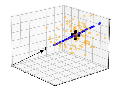
One is that if we have $n$ samples $x_1,…,x_n$, we can move to $\mathbb{R}^n$ by packaging $x=(x_1,…,x_n)$. Let $v=(1,1,…,1)$, the vector of all 1s. Note that the projection of two vectors is $\text{proj}_v x = (\frac{v\cdot x}{|v|^2})v$. In this case, $|v|^2 = n$ and $v\cdot x = \sum^n_{i=1} x_i$. So then in our situation, $(v\cdot x)/|v|^2 = \bar{x}$, the sample mean. Thus, computing the mean is related to projecting $x$ onto $(1,1,…,1)$.

On the other hand, let $w=x-\text{proj}_v x$. The vectors $x,v,w$ form a right triangle and $w$ is perpendicular to $v$. That is, $w \in \langle v\rangle^\perp$. Note that $|w|^2 = |x- \bar{x} v|^2 = \sum^n_{i=1} (x_i-\bar{x})^2$ and so $w$, if we scale it, will equal the standard deviation.

Let’s visualize this with $n=3$ samples. Suppose I generate 3 observations 100 times from a given distribution and plot them as $x=(x_1,x_2,x_3)$. These will form a cloud of points centered roughly around the vector determined by the true mean $(\mu,\mu,\mu)$. This is shown below; the yellow points represent each of the 3 observations put into a vector. We can project the yellow points onto the vector of ones $v$ (denoted below by $\vec{1}$) to get the sample mean for each. These are shown in blue. The big black plus is $(\mu,\mu,\mu)$; we don’t know its exact values but it makes sense that it should be at the center of the blue points. So the expected value $E[\bar{x}]=\mu$ which makes $\bar{x}$ and unbiased indicator of $\mu$.

On the other hand, to predict the true variance $\sigma^2$, we would need to know $\mu$. We don’t actually know $\mu$ but what we do know is that since $\bar{x}$ and $\mu$ lie on the same line spanned by $v$, projecting to the orthogonal complement would then send $\bar{x}$ and $\mu$ to the same point, namely to $0 \in U:=\langle v \rangle^\perp$. We can project all the yellow points into $U$ as well to get a new dataset with a known expected value of 0.

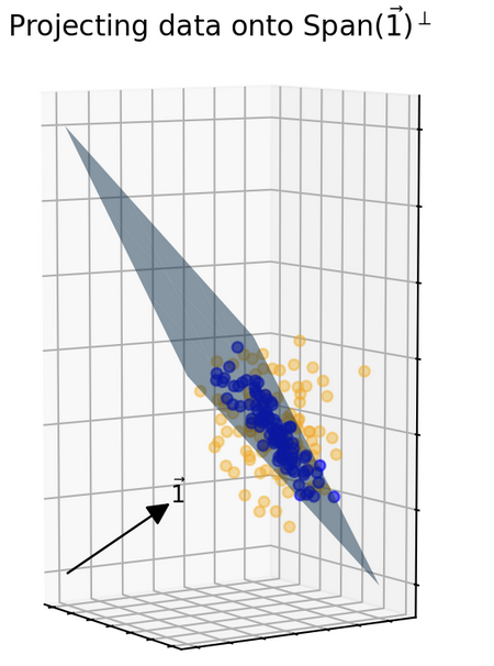
In general, if $y \in \mathbb{R}^k$ and the mean is 0 as we have here, then $\frac{1}{k}|y|^2$ is an unbiased indicator for $\sigma^2$. This is because $E(\frac{1}{k}|y|^2 )=\frac{1}{k}E(\sum^k y^2_i)= \frac{1}{k}\sum^k E(y^2_i)=\frac{1}{k}(k \sigma^2)=\sigma^2$. Well, our new data points are in $U \cong \mathbb{R}^2$ so $k=2$.

More generally, if we had general $n$, then to get an unbiased indicator, we’ll divide by $n-1 = \dim U$; this is Bessel’s correction.

In linear regression, since we assume the errors are normally distributed and also the samples are independent, we can then get a maximum likelihood function that is simply a product of many Gaussians. If we take the log of it, what comes out is just a quadratic form which is related to dot products. Since dot products are related to projection, we find that linear regression can be interpreted as projections and the simplest case of it is what we described above where we project just to a single vector. With linear regression, we’ll project into a $p+1$ dimensional subspace and the orthogonal complement has dimension $n-(p+1)$. The $p+1$ counts the degrees of freedom and we would see that terms for unbiased indicators contain $1/(n-p-1)$.

Let’s do this more rigorously. If we have $n$ labeled data points (labeled with $y$) and $p$ features, let $X$ be the $n \times p$ design matrix and $\beta$ will be a vector of $p$ coefficients. Then $y = X\beta +\epsilon$ where $\epsilon \sim N(0,\sigma^2 I_n)$ is normally distributed error. One way to compute the best estimate of $\beta$ is to use a matrix $H=X(X^\top X)^{-1} X^\top$ (the derivation just requires some consideration of minimizing some distance which uses projection which we can talk about with an inner product and some adjoints). $H$ is the matrix which projects onto the column space of $X$ and our predictions $\hat{y} = Hy$ need to use the labels. The residuals are $r = y- \hat{y} = (I-H)y$. Note that $I-H$ is the identity matrix minus a projection matrix which itself is also a projection matrix of rank $n-p$. Any projection matrix $P$ satisfies $P^2=P$. Hence, the residual sum of squares $\text{RSS} = r^\top r = y^\top (I-H)y$. As it turns out the distribution $\text{RSS}/\sigma^2 \sim \chi^2_{n-p}$ is a chi-squared distribution.

This is because, since the error is normally distributed, $r\sim N(0,\sigma^2(I-H))$ and we get a quadratic form $r^\top r = \epsilon^\top (I-H)\epsilon$. Now, any projection matrix $P$ of rank $k$ has a nice factorization $P = Q^\top I_k Q$ where $I_k$ is a matrix with 1 in the first $k$ diagonal entries and 0 everywhere else. That is, we can basically do a change of coordinates to make the subspace that $P$ projects to, a standard $k$-dim subspace. Moreover, we can keep the coordinates orthogonal because the transformation just needs to do some rotations in space. Okay, then $\epsilon^\top P \epsilon = (Q\epsilon)^\top I_{n-p}(Q\epsilon)$. But now, normal distributions are invariant under orthogonal transformations! So $Q\epsilon \sim N(0,\sigma^2 I_n)$ is still normally distributed. Thus, $(Q\epsilon)\top I_{n-p}Q\epsilon$, when you multiply things out, is $\sigma^2\sum^{n-p}Z^2_i$ where $Z_i$ are independent and identically distributed variables all drawn from $N(0,1)$.

But the sum of squared normal standard deviations, by definition, is just $\chi^2_{n-p}$. Since $E[Z^2_i] = \text{Var}(Z_i) + (E[Z_i])^2 = 1^2 + 0$, then $E[\chi^2_{n-p}] = n-p$. So $E[\text{RSS}/\sigma^2] = E[\chi^2_{n-p}]=n-p$ and hence, $\sigma^2 = \frac{1}{n-p}E[\text{RSS}]$. Hence, $s^2 = \frac{1}{n-p}\text{RSS}$ is an unbiased estimator of the variance.

Method of Moments

The $k$th moment of a random variable $X$ is $\mu_k = E[X^k]$. If $X_1,…,X_n$ are iid random variables, the $k$th sample moment is defined as $\hat{\mu}_k = \frac{1}{n}\sum^n_{i=1}X^k_i$.

The 1st sample moment is then just $\hat{\mu}_1=\bar{X}$, the sample mean which we can use to estimate the true mean $\mu$. Also, note that $\hat{\mu}_2-\hat{\mu}_1^2 = \frac{1}{n}\sum^n_{i=1}X^2_i - \bar{X}^2$ is an estimate for the true variance $\sigma^2$. These sample moment estimates are a method for estimating true population parameters and thus, the is called method of moments. We’ll return to this in a moment (horrible pun) but let’s introduce a few more definitions and results.

The moment generating function for a random variable $X$ is $M_X(s):=E[e^{sX}]$. If $X$ is a continuous random variable with a probability density function $f$, then $M_X(s)=\int^\infty_{-\infty}e^{sx}f(x)\,dx$. It may be that for many values of $s$, this diverges. But the main use is for its derivatives. Observe that the two-sided Laplace transform of $f$ is $\mathcal{L}{f}(s)=\int^\infty_{-\infty}e^{-sx}f(x)\,dx$ and so $M_X(s)=\mathcal{L}{f}(-s)$. The characteristic function on the other hand, is $\varphi_X(t) = E[e^{itX}] = \mathcal{F}{f}(-t)$ which is built from the Fourier transform.

Note that $\frac{d^n}{ds^n}M_X(s)|_{s=0} = \int^\infty_{-\infty}x^n f(x)\,dx$. The integral value here is the $n$ th moment of $X$. Note that for $n=0$, the answer is just 1 because that’s the total probability. For $n=1$, it is the expected value of $X$, $n=2$, it is a part of the definition for variance. And if re For $n=3$, it measures skewedness (symmetric distributions have 0 skewedness), for $n=4$, it measures kurtosis or “tailedness.”

So what’s the big deal about moments and moment generating functions?

Proposition: If $X,Y$ are random variables such that $M_X(s)=M_Y(s)$ for all $s$, then the cumulative distribution functions $F_X(x)=F_Y(x)$ for all $x$. So this means $X,Y$ have the same distribution.

Proposition: For a distribution of probability on a bounded interval, the collection of all the moments (of all orders, from 0 to $\infty$) uniquely determines the distribution. So in fact, we just need a countable collection of numbers to determine a distribution on a bounded interval. But this is not true for unbounded intervals.

So one of the useful things about moments is that in bounded cases, they can determine the distribution completely. But even if not, they are still useful. Let’s return to method of moments. The Central Limit Theorem (CLT) tells us that for large enough $n$, the distribution for $\bar{X}$ (viewed as a random variable in its own right) converges to $N(\mu,\sigma^2/n)$. Here, the 2nd entry is the variance, not the standard deviation. Different authors choose to denote the variance vs. standard deviation.

A sensible question to ask, in light of CLT, is: “Does the sample variance $s^2$ converge to a distribution as $n \to \infty$?” Above with Bessel’s inequality, we saw that to be unbiased, we use $s^2 = \frac{1}{n-1} \sum^n (X_i - \bar{X})^2$. Unforunately, we do not have a result as powerul as the Central Limit Theorem which assumed we could begin with any parent distribution from which we draw $n$ independent samples. However, if we begin with $N(\mu,\sigma^2)$ as our parent distribution, we can say something about how $s^2$ is distributed.

To address this point, let’s introduce the $\chi^2$ distribution. Let $Z\sim N(0,1)$. Then $\chi^2_1 \sim Z^2$ is the $\chi^2$ distribution with 1 degree of freedom. If $Z \sim N(\mu,\sigma^2)$, then $(Z-\mu)^2/\sigma^2 \sim \chi^2$.

If $U_1,…,U_n$ are all independent $\chi^2$ distributions with 1 degree of freedom, then $\chi^2_n=V=\sum U_i$ is called the $\chi^2$ distribution with $n$ degrees of freedom and $\sqrt{V}$ is called the $\chi$ distribution with $n$ degrees of freedom. The expected value of $\chi^2_n$ is $n$ and the variance is $2n$. When $n=3$, then $\sqrt{V}$ is an example of a Maxwell-Boltzmann distribution to describe the velocity of gas molecules in an idealized gas.

Anyways, observe that $\frac{1}{\sigma^2}\sum^n(X_i-\mu)^2 = \sum^n (\frac{X_i-\mu}{\sigma})^2 \sim \chi^2_n$. But also, $\frac{1}{\sigma^2}\sum^n(X_i-\mu)^2 = \frac{1}{\sigma^2} \sum^n ((X_i-\bar{X})+(\bar{X}-\mu))^2$. Interestingly, all the cross terms (the ones in grouped in the parentheses) cancel. So what we get in the end is $\frac{1}{\sigma^2}\sum^n(X_i-\mu)^2=(\frac{\bar{X}-\mu}{\sigma/\sqrt{n}})^2+ \frac{1}{\sigma^2}\sum^n(X_i-\bar{X})^2$.

This is of the form $W=U+V$ where $U$ and $V$ are independent. Thus, the moment generating functions have the relationship: $M_W=M_U M_V$. We see that $W \sim \chi^2_n$ and by CLT we also have $V\sim \chi^2_1$, then $U \sim \chi^2_{n-1}$. Hence, $s^2 \sim \frac{\sigma^2}{n-1}\chi^2_{n-1}$.

If you look at a graph of $\chi^2_{n-1}$, you’ll note that it is not symmetric about its expected vaule of 0. Thus, if we form a confidence interval, it will not be symmetric about $s^2$. The interval is $(\frac{ns^2}{\chi^2_{n-1}(\alpha/2)},\frac{ns^2}{\chi^2_{n-1}(1-\alpha/2)})$ where $\chi^2_{n-1}(\alpha/2)$ is the value such that $P(X<\chi^2_{n-1}(\alpha/2)) = \alpha/2$. Similarly, $P(X<\chi^2_{n-1}(1-\alpha/2)) = 1-\alpha/2$.

However, for $\bar{x}$, those confidence intervals are symmetric because the distribution in question is the normal distribution which is symmetric.

Having introduced $\chi^2$, we can also introduce the $t$-distribution with $k$ degrees of freedom. Let $Z\sim N(0,1)$ and $U_k \sim \chi^2_k$; these are assumed to be independent. Then $T_k \sim \frac{Z}{\sqrt{U_k/k}}$ which is a symmetric distribution; we have equal chance from $Z$ of being to the left and right of the mean 0 and we divide by something positive that is independent of $Z$. One thing to be careful about is that the PDF of $T_k$ is not the quotient of the PDFs of $Z$ and $\sqrt{U_k/k}$. If it were, it wouldn’t be symmetric. So if $U,V$ are independent distributions, in general $\text{PDF}(UV) \neq \text{PDF}(U)\cdot \text{PDF}(V)$.

Lastly, the $F$-distribution is a ratio: $F_{d_1,d_2}\sim \frac{U_{d_1}/d_1}{U_{d_2}/d_2}$. Here, $d_1,d_2$ are degrees of freedom. These $t$-distributions appear when we don’t have that many samples and so may see more extreme tails; it is sometimes called Student’s $t$-distribution because there was a statistician who used the pen name “Student.” He worked at a beer company and did not want to reveal his identity as that might reveal some trade secrets about the company.

The $F$-distribution is named after Fisher. It’s often used when we want to compare two things. For instance, maybe we have a full linear model and want to know how well a reduced linear model does in comparison. Or in ANOVA (analysis of variance), we might have 5 medical treatments and want to study the ratio of variance between medical treatments and variance within treatments. If this ratio (called an $F$-statistic) is large, then that indicates that the different treatments are likely to give different results, not merely because there is a lot of variation for any particular treatment.

Example: The following example is based on a very clear answer given by Steven Gubkin in stats.stackexchange. Steven also gave another answer on finding the PDF for the $F$-distribution by studying the unit sphere $S^{d_1+d_2-1}\subset \mathbb{R}^{d_1+d_2}$ and then projecting into the spheres $S^{d_1-1}$ and $S^{d_2-1}$ in the respective subspaces. I won’t discuss this derivation here but it’s quite nice. Before moving on, let me recall some definitions.

Errors: When we study some parameter for a population, there is a true expected value and the observations we sample will (usually) deviate from that true expected value. The difference is called the error and the error forms a distribution. We often assume that error is normally distributed. e.g. in linear regression, there is some “true” $\beta$ of parameters so that $y_{obs}=X\beta+\epsilon$.

Residuals: On the other hand, we can take samples and develope a model to try and make predictions. The difference between the predicted values and the observations is the residual. e.g. in linear regression, we have a $\hat{\beta}$ that we find from trying to fit our model to our samples. We then have $y_{obs}-X\hat{\beta}$ are the residuals.

Now suppose we have some data which satisfies the assumptions needed to run linear regression. That is, we assume there’s a linear relationship between some features $X$ and outcome $Y$ and that the errors are independent and all drawn from a normal distribution $N(0,\sigma^2 I)$ (so the variance doesn’t change between different data points). To proceed, let’s first state a very useful theorem.

Theorem: If $X \sim N(0,\sigma^2I)$ is normally distributed on an inner product space $V$, then for any subspace $U\subset V$ we have that $\text{Proj}_U(X)$ and $\text{Proj}_{U^\perp}(X)$ are independent and are both normally distributed with the same variance $\sigma^2$.

Alright, now the $F$-statistic allows us to make a comparison. We have an ambient space $\mathbb{R}^n$ and we have two models that we want to fit to some data. One model uses $p$ parameters which we call the full model and the other uses $q<p$ parameters which we call the reduced model.

The full model is $Y=\beta_0+\beta_1X_1+…+\beta_q X_q+\beta_{q+1}X_{q+1}+…+\beta_pX_p$ while the reduced model is $Y=\beta_0+\beta_1X_1+…+\beta_q X_q$; so it says $\beta_{q+1}=…=\beta_p=0$.

So let $F=\text{Span}\{1,x_1,…,x_p\}$ and $R=\text{Span}\{1,x_1,…,x_q\}$. The hypothesis test we set up is:

Null hypothesis: the true values are described by the reduced model. Alternative hypothesis: the true values are described by the full model.

Here’s a geometric picture; we depict $R$ as a line and $F$ as a plane but they are larger linear subspaces in general.

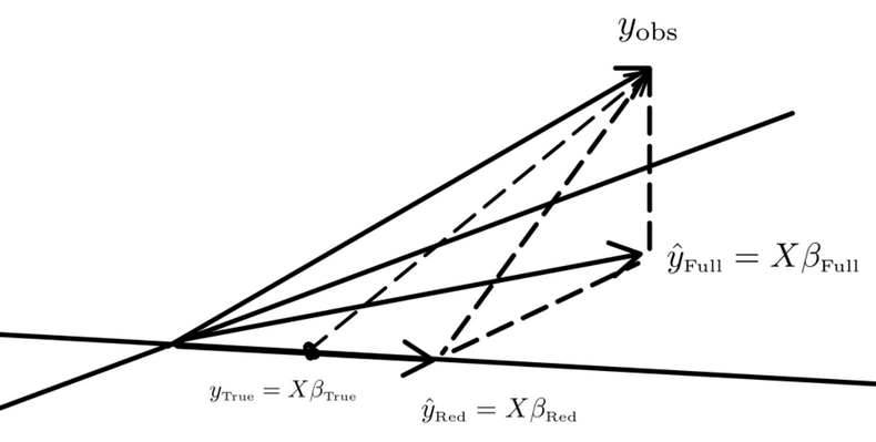
The picture depicts the null hypothesis that the true value is in the space $R$ that is spanned by the reduced model. The error is $y_{obs}-y_{True} \in R^\perp$ which is drawn from $N(0,\sigma^2 I)$. Also, $y_{obs}-\hat{y}_{Red} \in R^\perp$, $y_{obs}-\hat{y}_{Full}\in F^\perp$ and $\hat{y}_{Full}-\hat{y}_{Red} \in F\cap R^\perp$.

Under the null hypothesis, if we project $y_{obs}-y_{True}$ into $F$, I believe we obtain a random vector which aligns with $\hat{y}_{Full}-\hat{y}_{Red}$ and the theorem above tells us that that this is also normally distributed on $F \cap R^\perp$ (which has dimension $p-q$) with variance $\sigma^2$. Also, $y_{obs}-\hat{y}_{Full}\in F^\perp$ is normally distributed; $\dim F^\perp = n-p-1$; the extra 1 is from the span containing a 1 for $\beta_0$.

Then $|\hat{y}_{Full}-\hat{y}_{Red}|^2$ is a sum of squares of $p-q$ iid terms all with variance $\sigma^2$. So $|\hat{y}_{Full}-\hat{y}_{Red}|^2 \sim \sigma^2 \chi^2_{p-q}$ and $|y_{obs}-\hat{y}_{Full}|^2\sim \sigma^2 \chi^2_{n-p-1}$ these are independent as they are in orthogonal spaces. Then the $F$ distribution is to built from a ratio of these multiplied by another fraction that uses the dimensions (see above for the definition): $\frac{n-p-1}{p-q} \frac{|\hat{y}_{Full}-\hat{y}_{Red}|^2}{|y_{obs}-\hat{y}_{Full}|^2} \sim F(p-q,n-p-1)$.

Note: I changed the notation a bit so that I don’t have a long subscript for the $F$-distribution.

If $\theta$ is the angle between $\hat{y}_{Full}-\hat{y}_{Red}$ and $y_{obs}-\hat{y}_{Full}$, then the $F$-distribution is, up to a constant, just $\cot^2(\theta)$. If the angle is very small, then $\cot^2(\theta)$ is large. But also, a small angle means that $y_{obs}$ is very close to $\hat{y}_{Full}$ which would be very strange, assuming the Null Hypothesis which says that it should be $y_{obs}$ and $\hat{y}_{Red}$ that are closer.

Also, by the Pythagorean Theorem, $|\hat{y}_{Full}-\hat{y}_{Red}|^2 + |y_{obs}-\hat{y}_{Full}|^2 = |y_{obs}-\hat{y}_{Red}|^2$ so sometimes we see the numerator of the $F$-distribution above replaced by an appropriate different of squares.

Maximum Likelihood Estimator

Suppose we have $n$ samples $X_1,…,X_n$ and we compute a statistic $\hat{\theta}$ from the samples. We can then ask, what’s the most likely true value $\theta_0$ which would give us these samples? The way to find this is by simple calculus: we find the joint PDF for these samples given $\theta$ and then differentiate with respect to $\theta$, then find a critical point; hopefully it’s a global max which then says it’s the most likely parameter to give rise to our samples.

Example 1: Suppose we have $n$ samples independently and identically drawn from a (discrete) Poisson distribution whose PDF is $f(k)=\lambda^k e^{-\lambda}/k!$. Then the joint distribution is $L(\lambda)=e^{-n\lambda} \lambda^{\sum^n k_i}/k_1!…k_n!$ which, when we take the log, will be easier to work with: $\log L(\lambda) = -n\lambda + \log(\lambda) \sum^n k_i-\sum^n \log(k_i!)$.

Differentiating with respect to $\lambda$ and setting equal to 0 (the last term goes away), we get $\frac{1}{\lambda} \sum^n k_i = n$ and thus, $\lambda = \frac{1}{n}\sum^nk_i$ which is the average of the samples which agrees with the 1st sample moment of $\bar{k}$.

Example 2: Let’s draw $n$ samples $X_1,…,X_n$ from a uniform distribution on $[0,b]$ where $b$ is unknown. The 1st moment is $\mu_1 = b/2$ and so the 1st sample moment is $\hat{\mu}_1 = \bar{X}=\hat{b}/2$ and so the method of moments predicts $\hat{b}_{MOM}=2\bar{X}$. On the other hand, using maximum likelihood estimates, we’d find that the best estimate there is that $\hat{b}_{MLE}=\max{X_1,…,X_n}$. So the two methods differ.

Also, $E[\hat{b}_{MOM}]=2E[\bar{X}] = b$ so this is an unbiased estimator. However, $E[\hat{b}_{MLE}]=E[\max{X_1,…,X_n}] = \frac{1}{b^n}\int_{[0,b]^n} \max{X_1,…,X_n}\,dV$

This integral can be broken into $n$ pieces on various simplices of the hypercube $[0,b]^n$ where on each pieces, we just integrate one of the $X_i$. The results are all the same so we really just need to find $\frac{n}{b^n}\int_{n-\text{simplex}} X_1\, dV$. This is still rather complicated to compute but it comes out to be $\frac{n}{n+1}b$ which shows we have a biased estimator.

Recall that we say an estimator $\hat{\theta}_n$ (built from $n$ samples) is consistent if, as the number of samples $n \to \infty$, the sequence of estimator sampling distributions converges (in measure) towards the true parameters value. This means they converge to a Dirac delta type of distribution concentrated on $\theta$. In our case, $\hat{b}_{MLE}$ is a consistent estimator for this uniform distribution example.

In fact: Theorem 1: Under appropriate smoothness conditions on the PDF $f$ of a continuous random distribution $D$, the maximum likelihood estimate $\hat{\theta}_n$ for a parameter $\theta$ of $n$ samples independently and identically drawn from $D$ is consistent. We can formulate this as saying that for any $\epsilon >0$, $P(|\hat{\theta}_n-\theta|>\epsilon) \to 0$.

To prove this, let’s begin with a lemma.

Lemma: Define $I(\theta)=E[(\partial_\theta \log f(X|\theta))^2]$. Under appropriate smoothness conditions on $f$, $I(\theta) = -E[\partial^2_\theta \log f(X|\theta)]$. That is the expected value of the square of the 1st partial derivative of the log of $f$ is equal to the negative expected value of the 2nd partial derivative of the log of $f$.

Proof: For the sake of decluttering notation, I’ll just write $f$ instead of $f(X|\theta)$ for the most part. Then note that $\int_\Omega f\, dx =1$ which means $\partial_\theta \int_\Omega f\, dx = 0$. Also, observe that $\partial_\theta \log(f) = f’/f$ so $\partial_\theta f = f\cdot \partial_\theta \log(f)$. Combining these two facts, we have: $0=\partial_\theta \int_\Omega f\, dx = \int_\Omega \partial_\theta f\, dx = \int_\Omega f\partial_\theta \log(f)\, dx$.

Here, we need some smoothness assumptions on $f$ in order to interchange differentiation with integration. Applying another $\partial_\theta$ to the previous equation and using product rule, we have: $0=\partial_\theta \int_\Omega f\partial_\theta \log(f)\, dx = \int_\Omega f(\partial_\theta \log(f))^2\, dx + \int_\Omega f\partial^2_\theta \log(f)\, dx$.

This is a sum of expected values and the probability measure is $f\, dx$. So we’ve shown $E[(\partial_\theta \log f(X|\theta))^2]=-E[\partial^2_\theta \log f(X|\theta)]$. $\square$

Theorem 2: Let $\hat{\theta}_n$ be the maximum likelihood estimate of some population parameter whose true value is $\theta_0$. Under the same smooth conditions on $f$ as Thm. 1 and also that the true value $\theta_0$ is a critical point, not a boundary point of the maximum likelihood function, then $\sqrt{nI(\theta_0)}(\hat{\theta}_n-\theta_0)$ converges in distribution to the standard normal distribution $N(0,1)$.

Proof: Let’s write the log likelihood as $\ell(\theta)$. A Taylor series expansion around $\theta_0$ shows that $\ell(\theta) \approx \ell(\theta_0)+\ell’(\theta_0)(\theta-\theta_0) + \frac{\ell’’(\theta_0)}{2!}(\theta-\theta_0)^2$.

Differentiating, we have $\ell’(\theta) \approx \ell’(\theta_0)+\ell’’(\theta_0)(\theta-\theta_0)$. Now, $\hat{\theta}$ is a critical point so if we plug it in, we have $0 = \ell’(\hat{\theta}) \approx \ell’(\theta_0)+\ell’’(\theta_0)(\hat{\theta}-\theta_0)$. Then $\hat{\theta}-\theta_0 \approx -\ell’(\theta_0)/\ell’’(\theta_0)$.

Let’s rewrite this as $n^{1/2}(\hat{\theta}-\theta_0) \approx \frac{-n^{-1/2}\ell’(\theta_0)}{n^{-1}\ell’’(\theta_0)}$.

The expected value of the numerator was computed in the lemma and we saw that it’s 0. It’s variance is exactly what we defined to be $I(\theta_0)$.

Anyways, the denominator, on the other hand, equals $\frac{1}{n}\ell’’(\theta_0) = \frac{1}{n}\sum^n \partial^2_\theta \log(f)(\theta_0)$. The Law of Large Numbers tells us that this average approaches the expected value as $n \to \infty$ which we write as $E[\partial^2_\theta \log(f)(\theta_0)] = -I(\theta)$. Therefore, as $n$ grows, our approximation above becomes $\sqrt{n}(\hat{\theta}-\theta_0) \approx n^{-1/2}\ell’(\theta_0)/I(\theta_0) \to 0$ as $n \to \infty$. Thus, the expected value of the LHS is approximately 0.

Moreover, the variance of the LHS is approximately the expected value of the square of the RHS (since subtracting off the square of the expected value is to subtract $0^2$). But this, which we noted above about the numerator, is just $I(\theta_0)/I(\theta_0)^2$. So the variance of $\hat{\theta}-\theta_0 \approx \frac{1}{nI(\theta_0)}$. Now, $\ell’(\theta_0) = \sum^n \partial_\theta \log(f)(\theta_0)$ is a sum of iid so we can apply the Central Limit Theorem to it. Thus, $\sqrt{nI(\theta_0)}(\hat{\theta}-\theta_0)$ converges to the standard normal distribution. Put into other words $\hat{\theta}_n$ converges to $N(\theta_0, 1/nI(\theta_0))$ where the 2nd entry is the variance. So $\hat{\theta}_n$ is asymptotically unbiased. $\square$

Let’s define $\text{Bias}(\hat{\theta})=E[\hat{\theta}]-\theta$ where $\theta$ is the true parameter (I got tired of typing $\theta_0$). Also, the mean squared error is defined as $\text{MSE}(\hat{\theta}) = E[(\hat{\theta}-\theta)^2]$ which we can show equals $\text{Var}(\hat{\theta})+\text{Bias}(\hat{\theta})^2$. Importantly, this is when we’re trying to estimate a single number: the population parameter.

Also, when we have large $n$, the confidence interval for $\theta$ is $\left(\hat{\theta}-\frac{z(\alpha/2)}{\sqrt{nI(\hat{\theta})}},\hat{\theta}+\frac{z(\alpha/2)}{\sqrt{nI(\hat{\theta})}}\right)$. This one is symmetric because, as our theorem above showed that for large $n$, $\hat{\theta}$ converges to a normal distribution.

Above, we’re trying to estimate the population parameter. But if we’re trying to estimate a target such as $Y = f(x) +\epsilon$ which is split into a deterministic and random part $\epsilon \sim N(0,\sigma^2)$, then we might try to estimate $f(x)$ using a model $\hat{f}(x)$. Then the expected squared error at $x$ is $E[(\hat{f}(x)-f(x))^2] = (E[\hat{f}(x)] - f(x))^2 + \text{Var}(\hat{f}(x)) + \sigma^2$ which is the bias of the estimator $\hat{f}(x)$ squared plus variance of $\hat{f}(x)$ plus irreducible noise.